Working With tidycensus

library(griddy)
library(dplyr)
library(tidyr)

This article is a website-only template for ACS workflows: it requires a Census API key and live data, so it is rendered on the pkgdown site when the key is set and skipped otherwise. It does not ship with the installed package.

library(tidycensus)
library(sf)

## Warning: package 'sf' was built under R version 4.5.2

## Linking to GEOS 3.13.0, GDAL 3.8.5, PROJ 9.5.1; sf_use_s2() is TRUE

library(sfdep)

years <- c(2012, 2017, 2022)

acs <- purrr::map_dfr(years, function(y) {
  get_acs(
    geography = "tract",
    variables = "B19013_001",
    state = "CA",
    county = "San Francisco",
    year = y,
    survey = "acs5",
    geometry = TRUE
  ) |>
    transmute(
      GEOID,
      year = y,
      median_income = estimate,
      geometry
    ) |>
    filter(is.finite(median_income))
})

## Getting data from the 2008-2012 5-year ACS

## Downloading feature geometry from the Census website.  To cache shapefiles for use in future sessions, set `options(tigris_use_cache = TRUE)`.

## Getting data from the 2013-2017 5-year ACS

## Downloading feature geometry from the Census website.  To cache shapefiles for use in future sessions, set `options(tigris_use_cache = TRUE)`.

## Getting data from the 2018-2022 5-year ACS

## Downloading feature geometry from the Census website.  To cache shapefiles for use in future sessions, set `options(tigris_use_cache = TRUE)`.

geography <- acs |>
  filter(year == max(year)) |>
  filter(!st_is_empty(geometry)) |>
  arrange(GEOID)

common_ids <- acs |>
  st_drop_geometry() |>
  count(GEOID) |>
  filter(n == length(years)) |>
  pull(GEOID) |>
  intersect(geography$GEOID)

panel <- acs |>
  filter(GEOID %in% common_ids) |>
  st_drop_geometry() |>
  left_join(select(geography, GEOID, geometry), by = "GEOID") |>
  st_as_sf()

geography <- geography |>
  filter(GEOID %in% common_ids) |>
  arrange(GEOID) |>
  mutate(
    nb = st_contiguity(geometry, queen = TRUE),
    wt = st_weights(nb, allow_zero = TRUE)
  )

## Warning: There was 1 warning in `stopifnot()`.
## ℹ In argument: `nb = st_contiguity(geometry, queen = TRUE)`.
## Caused by warning in `spdep::poly2nb()`:
## ! neighbour object has 2 sub-graphs;
## if this sub-graph count seems unexpected, try increasing the snap argument.

classes <- classify_dynamics(panel, GEOID, year, median_income, k = 5)
classic <- markov_dynamics(classes, GEOID, year, class)
spatial <- spatial_markov(panel, GEOID, year, median_income, geometry = geography, k = 5)
mobility <- rank_mobility(panel, GEOID, year, median_income)

plot_transition_matrix(classic)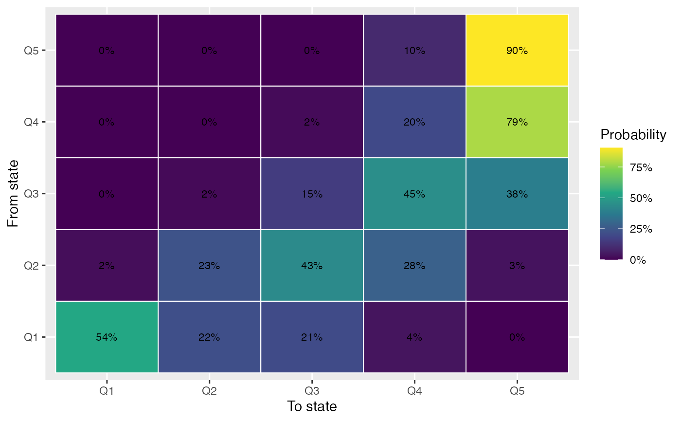

plot_spatial_markov(spatial)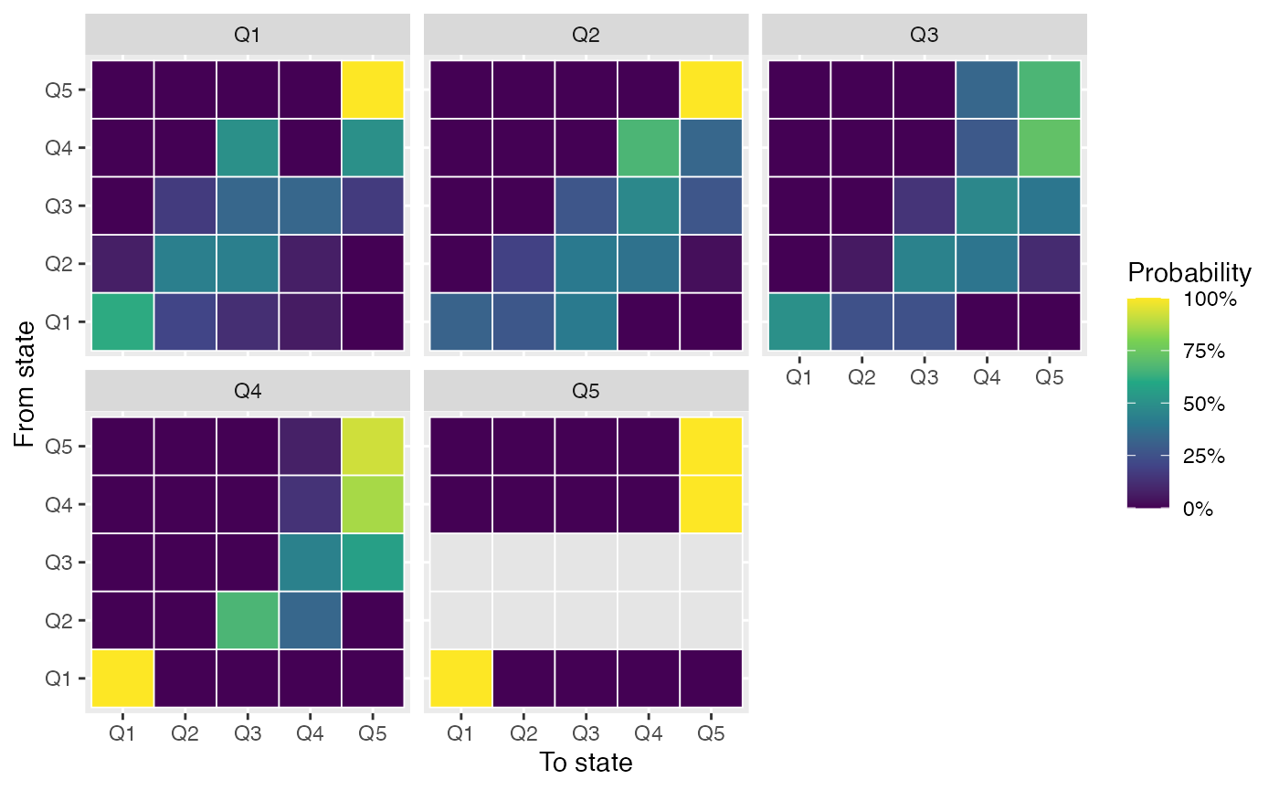

plot_rank_mobility(mobility)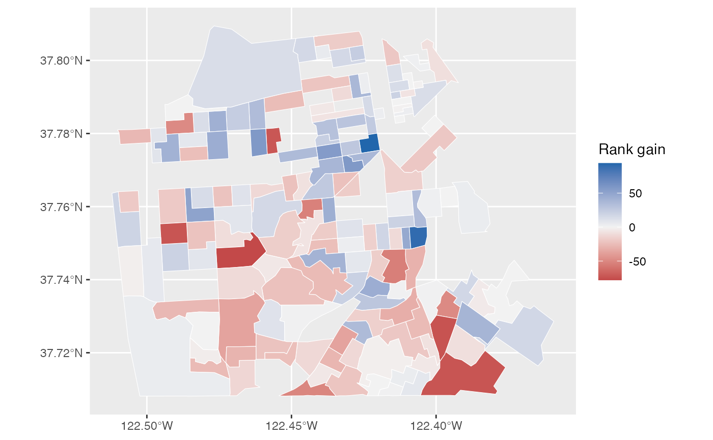

For package-ready examples, cache a small static panel instead of calling the API at build time.