Bayesian Surprise with Canadian Census Data (cancensus)
Source:vignettes/cancensus-workflow.Rmd
cancensus-workflow.RmdIntroduction
This vignette demonstrates how to use the
bayesiansurpriser package with Canadian Census data
accessed through the cancensus package. The cancensus
package provides access to Canadian Census data from 1996 through 2021
via the CensusMapper API.
Canadian Census data is a useful setting for Bayesian Surprise analysis because it provides:
- Comprehensive population data at multiple geographic levels
- Rich demographic and socioeconomic variables
- Consistent geography across Census years
- Both counts and rates for many variables
As with ACS examples, Census profile counts are best treated carefully. The surprise maps below model rates directly using distributional models. Funnel plots are used separately as diagnostics for how population or household counts affect the reliability of rates.
Prerequisites
You’ll need a CensusMapper API key from https://censusmapper.ca/users/sign_up
library(bayesiansurpriser)
library(cancensus)
library(sf)
library(ggplot2)
library(dplyr)

# Set your CensusMapper API key (do this once)
# set_cancensus_api_key("YOUR_KEY_HERE", install = TRUE)

# Optionally set a cache path for faster subsequent queries
# set_cancensus_cache_path("path/to/cache", install = TRUE)
Understanding cancensus Data Structure
Before diving into analysis, let’s understand the available datasets and variables.
# List available Census datasets
datasets <- list_census_datasets()
print(datasets %>% select(dataset, description))
# List regions for the 2021 Census
regions_2021 <- list_census_regions("CA21")
head(regions_2021 %>% filter(level == "CMA"))
Example 1: Low Income Rates by Census Division
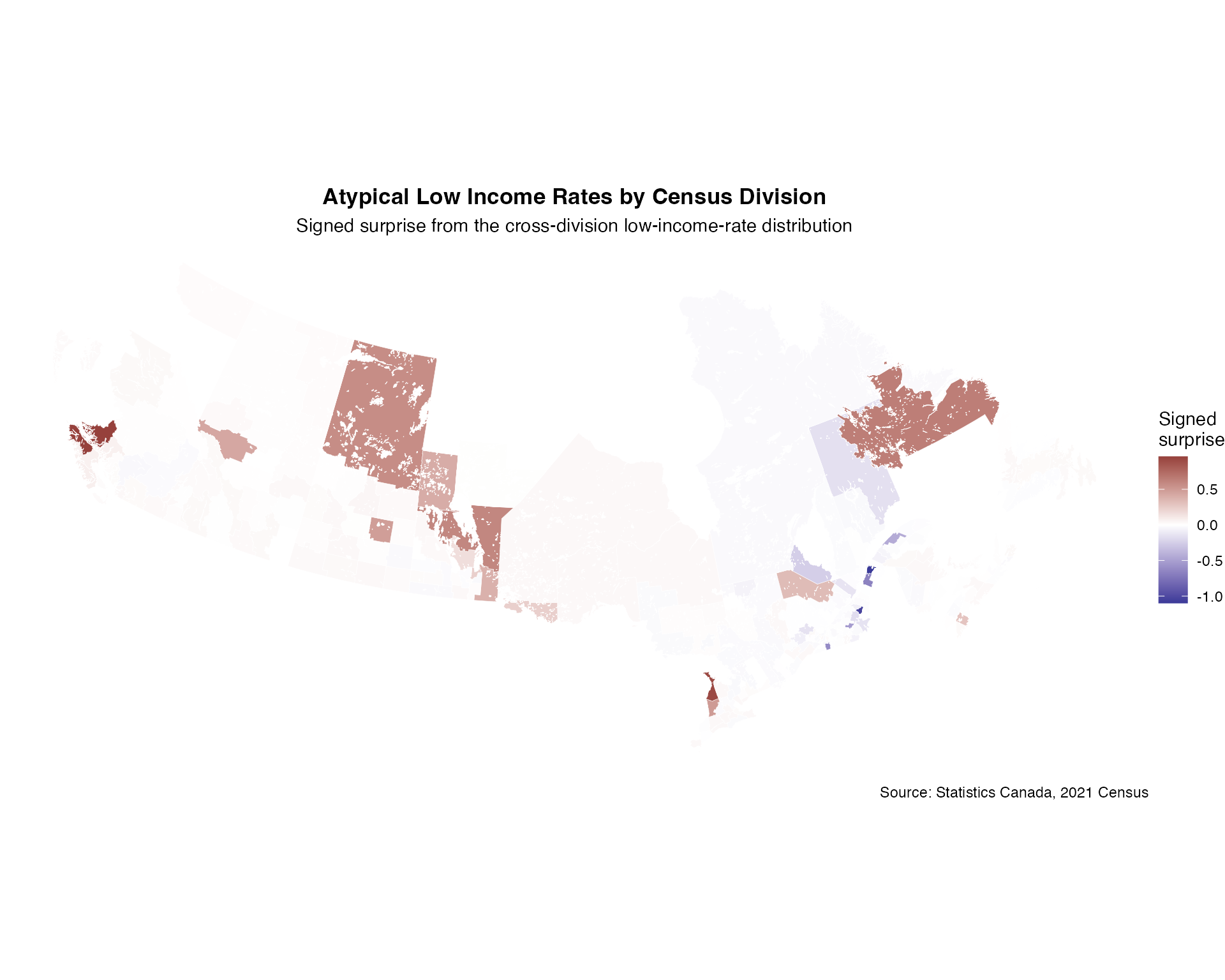
Let’s examine low income rates across Canada’s Census Divisions and identify which regions have atypical rates relative to the cross-division distribution.
Fetch Census Data
# Find relevant vectors for low income
# v_CA21_1085: Total - Low-income status in 2020
# v_CA21_1086: 0 to 17 years in low income
# v_CA21_1090: In low income

# Get low income data at the Census Division level for all of Canada
# Using labels = "short" for cleaner column names
income_data <- get_census(
  dataset = "CA21",
  regions = list(C = "01"),  # All of Canada
  vectors = c(
    total_pop = "v_CA21_1085",  # Total population for low income status
    low_income = "v_CA21_1090"   # Population in low income
  ),
  level = "CD",
  geo_format = "sf",
  labels = "short",
  quiet = TRUE
)

# Clean and filter
income_data <- income_data %>%
  filter(!is.na(total_pop) & !is.na(low_income)) %>%
  filter(total_pop > 0) %>%
  mutate(
    low_income_rate = low_income / total_pop
  )

head(income_data %>% st_drop_geometry() %>% select(GeoUID, `Region Name`, total_pop, low_income, low_income_rate))
#>   GeoUID           Region Name total_pop low_income low_income_rate
#> 1   1001 Division No.  1 (CDR)       4.3        3.9       0.9069767
#> 2   1002 Division No.  2 (CDR)       2.6        2.4       0.9230769
#> 3   1003 Division No.  3 (CDR)       2.3        1.6       0.6956522
#> 4   1004 Division No.  4 (CDR)       5.2        2.8       0.5384615
#> 5   1005 Division No.  5 (CDR)       3.4        3.0       0.8823529
#> 6   1006 Division No.  6 (CDR)       3.7        3.5       0.9459459
Compute Bayesian Surprise
# Compute surprise on the low-income-rate distribution.
income_surprise <- surprise(
  income_data,
  observed = low_income_rate,
  models = c("uniform", "gaussian", "sampled")
)

print(income_surprise)
#> Bayesian Surprise Map
#> =====================
#> Models: 3
#> Surprise range: 0.0012 to 1.0991
#> Signed surprise range: -1.0991 to 0.9596
#>
#> Simple feature collection with 276 features and 18 fields
#> Attribute-geometry relationships: constant (15), NA's (3)
#> Geometry type: MULTIPOLYGON
#> Dimension:     XY
#> Bounding box:  xmin: -133.1543 ymin: 41.7251 xmax: -52.61938 ymax: 62.58185
#> Geodetic CRS:  WGS 84
#> First 10 features:
#>    Shape Area Type Households Population 2016 GeoUID PR_UID Population
#> 1    9104.580   CD     117178          270348   1001     10     271878
#> 2    5915.569   CD       8891           20372   1002     10      19392
#> 3   19272.107   CD       6342           15560   1003     10      13920
#> 4    7019.972   CD       9196           20387   1004     10      19253
#> 5   10293.762   CD      17967           42014   1005     10      40396
#> 6   16043.377   CD      16489           38345   1006     10      37339
#> 7    9598.370   CD      14867           34092   1007     10      33044
#> 8    9234.941   CD      15385           35794   1008     10      33940
#> 9   13209.476   CD       6640           15607   1009     10      14733
#> 10 191691.086   CD       9518           24639   1010     10      24332
#>    Households 2016 Dwellings Dwellings 2016                  name
#> 1           112620    135137         131336 Division No.  1 (CDR)
#> 2             8737     11551          11497 Division No.  2 (CDR)
#> 3             6773      8046           8289 Division No.  3 (CDR)
#> 4             9345     10900          11338 Division No.  4 (CDR)
#> 5            17890     20875          20924 Division No.  5 (CDR)
#> 6            16434     19498          19296 Division No.  6 (CDR)
#> 7            14571     20304          20097 Division No.  7 (CDR)
#> 8            15587     21721          21913 Division No.  8 (CDR)
#> 9             6689      9366           9346 Division No.  9 (CDR)
#> 10            9193     10941          10758 Division No. 10 (CDR)
#>              Region Name Area (sq km) total_pop low_income
#> 1  Division No.  1 (CDR)     9104.580       4.3        3.9
#> 2  Division No.  2 (CDR)     5915.569       2.6        2.4
#> 3  Division No.  3 (CDR)    19272.107       2.3        1.6
#> 4  Division No.  4 (CDR)     7019.972       5.2        2.8
#> 5  Division No.  5 (CDR)    10293.762       3.4        3.0
#> 6  Division No.  6 (CDR)    16043.377       3.7        3.5
#> 7  Division No.  7 (CDR)     9598.370       2.4        2.2
#> 8  Division No.  8 (CDR)     9234.941       2.6        1.6
#> 9  Division No.  9 (CDR)    13209.476       1.5        1.6
#> 10 Division No. 10 (CDR)   191691.086       2.0        2.8
#>                          geometry low_income_rate    surprise signed_surprise
#> 1  MULTIPOLYGON (((-52.79548 4...       0.9069767 0.030040863     0.030040863
#> 2  MULTIPOLYGON (((-54.64846 4...       0.9230769 0.028202690     0.028202690
#> 3  MULTIPOLYGON (((-55.8764 47...       0.6956522 0.015582828    -0.015582828
#> 4  MULTIPOLYGON (((-59.2948 47...       0.5384615 0.008926266    -0.008926266
#> 5  MULTIPOLYGON (((-58.26214 4...       0.8823529 0.032003269     0.032003269
#> 6  MULTIPOLYGON (((-55.27854 4...       0.9459459 0.024869967     0.024869967
#> 7  MULTIPOLYGON (((-53.74344 4...       0.9166667 0.028985389     0.028985389
#> 8  MULTIPOLYGON (((-54.24936 4...       0.6153846 0.002961314    -0.002961314
#> 9  MULTIPOLYGON (((-55.42497 5...       1.0666667 0.002981345     0.002981345
#> 10 MULTIPOLYGON (((-60.91505 5...       1.4000000 0.643186681     0.643186681
summary(income_surprise)
#>    Shape Area       Type       Households      Population 2016
#>  Min.   :   206.5   CD:276   Min.   :    780   Min.   :   2558
#>  1st Qu.:  1852.4            1st Qu.:   9506   1st Qu.:  21874
#>  Median :  3731.3            Median :  19418   Median :  42744
#>  Mean   : 18507.5            Mean   :  54030   Mean   : 126745
#>  3rd Qu.: 14803.9            3rd Qu.:  40004   3rd Qu.:  89067
#>  Max.   :707306.5            Max.   :1160892   Max.   :2731571
#>
#>     GeoUID             PR_UID            Population      Households 2016
#>  Length:276         Length:276         Min.   :   2323   Min.   :    834
#>  Class :character   Class :character   1st Qu.:  22034   1st Qu.:   9368
#>  Mode  :character   Mode  :character   Median :  45072   Median :  18056
#>                                        Mean   : 133404   Mean   :  50753
#>                                        3rd Qu.:  94928   3rd Qu.:  38072
#>                                        Max.   :2794356   Max.   :1112929
#>
#>    Dwellings       Dwellings 2016        name
#>  Min.   :    845   Min.   :    945   Length:276
#>  1st Qu.:  11466   1st Qu.:  11332   Class :character
#>  Median :  21558   Median :  20886   Mode  :character
#>  Mean   :  58718   Mean   :  55565
#>  3rd Qu.:  42987   3rd Qu.:  41316
#>  Max.   :1253238   Max.   :1179057
#>
#>                 Region Name   Area (sq km)        total_pop       low_income
#>  Division No.  1 (CDR):  4   Min.   :   206.5   Min.   : 1.10   Min.   :0.300
#>  Division No.  2 (CDR):  4   1st Qu.:  1852.4   1st Qu.: 2.50   1st Qu.:1.800
#>  Division No.  3 (CDR):  4   Median :  3731.3   Median : 3.10   Median :2.600
#>  Division No.  4 (CDR):  4   Mean   : 18507.5   Mean   : 3.26   Mean   :2.797
#>  Division No.  5 (CDR):  4   3rd Qu.: 14803.9   3rd Qu.: 3.70   3rd Qu.:3.600
#>  Division No.  6 (CDR):  4   Max.   :707306.5   Max.   :10.90   Max.   :9.400
#>  (Other)              :252
#>           geometry   low_income_rate     surprise        signed_surprise
#>  MULTIPOLYGON :276   Min.   :0.1818   Min.   :0.001157   Min.   :-1.099116
#>  epsg:4326    :  0   1st Qu.:0.6667   1st Qu.:0.007890   1st Qu.:-0.019145
#>  +proj=long...:  0   Median :0.8443   Median :0.021936   Median : 0.001403
#>                      Mean   :0.8367   Mean   :0.062956   Mean   : 0.007089
#>                      3rd Qu.:1.0000   3rd Qu.:0.031610   3rd Qu.: 0.025769
#>                      Max.   :1.4737   Max.   :1.099116   Max.   : 0.959614
#>
Visualize Surprising Regions
# Add surprise values to data
income_data$surprise <- get_surprise(income_surprise, "surprise")
income_data$signed_surprise <- get_surprise(income_surprise, "signed")

# Transform to Statistics Canada Lambert projection for better Canada visualization
income_data_lambert <- st_transform(income_data, "EPSG:3347")

# Plot Canada-wide
ggplot(income_data_lambert) +
  geom_sf(aes(fill = signed_surprise), color = "white", linewidth = 0.1) +
  scale_fill_surprise_diverging(name = "Signed\nsurprise") +
  labs(
    title = "Atypical Low Income Rates by Census Division",
    subtitle = "Signed surprise from the cross-division low-income-rate distribution",
    caption = "Source: Statistics Canada, 2021 Census"
  ) +
  theme_void() +
  theme(
    legend.position = "right",
    plot.title = element_text(hjust = 0.5, face = "bold"),
    plot.subtitle = element_text(hjust = 0.5)
  )
Identify Most Surprising Regions
# Top regions with positive signed surprise
high_income_surprise <- income_data %>%
  st_drop_geometry() %>%
  filter(signed_surprise > 0) %>%
  arrange(desc(surprise)) %>%
  select(`Region Name`, low_income_rate, total_pop, surprise) %>%
  head(10)

cat("Census Divisions with positive signed surprise:\n")
#> Census Divisions with positive signed surprise:
print(high_income_surprise)
#>              Region Name low_income_rate total_pop  surprise
#> 1  Mount Waddington (RD)        1.473684       3.8 0.9596140
#> 2            Bruce (CTY)        1.464286       2.8 0.9166387
#> 3  Division No. 10 (CDR)        1.400000       2.0 0.6431867
#> 4  Division No. 19 (CDR)        1.387755       4.9 0.5980193
#> 5  Division No. 18 (CDR)        1.378378       3.7 0.5653834
#> 6            Huron (CTY)        1.354839       3.1 0.4909450
#> 7  Division No. 10 (CDR)        1.350000       4.0 0.4769159
#> 8  Division No. 14 (CDR)        1.333333       2.7 0.4316586
#> 9  Division No. 21 (CDR)        1.323529       3.4 0.4069403
#> 10 Division No.  1 (CDR)        1.312500       3.2 0.3803817

# Top regions with negative signed surprise
low_income_surprise <- income_data %>%
  st_drop_geometry() %>%
  filter(signed_surprise < 0) %>%
  arrange(desc(surprise)) %>%
  select(`Region Name`, low_income_rate, total_pop, surprise) %>%
  head(10)

cat("\nCensus Divisions with negative signed surprise:\n")
#>
#> Census Divisions with negative signed surprise:
print(low_income_surprise)
#>                         Region Name low_income_rate total_pop  surprise
#> 1             Rivière-du-Loup (MRC)       0.1818182       2.2 1.0991165
#> 2               Robert-Cliche (MRC)       0.2000000       1.5 1.0416346
#> 3                  Kamouraska (MRC)       0.3000000       2.0 0.6692050
#> 4  Les Jardins-de-Napierville (MRC)       0.3125000       1.6 0.6151227
#> 5                 Les Sources (MRC)       0.3333333       3.0 0.5239340
#> 6                  La Matanie (MRC)       0.3529412       3.4 0.4386328
#> 7           Le Domaine-du-Roy (MRC)       0.4000000       2.5 0.2504012
#> 8              Les Appalaches (MRC)       0.4230769       2.6 0.1751860
#> 9  Sept-Rivières--Caniapiscau (CDR)       0.4285714       2.1 0.1594827
#> 10            Les Laurentides (MRC)       0.4333333       3.0 0.1465783
Example 2: Housing Analysis in Metro Vancouver
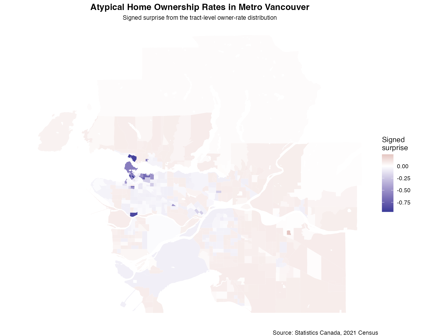
Let’s analyze owner-occupied housing rates at the Census Tract level within the Vancouver CMA.
# Get housing tenure data for Vancouver CMA
# v_CA21_4237: Total private households by tenure
# v_CA21_4238: Owner households

housing_data <- get_census(
  dataset = "CA21",
  regions = list(CMA = "59933"),  # Vancouver CMA
  vectors = c(
    total_hh = "v_CA21_4237",  # Total households
    owner_hh = "v_CA21_4238"   # Owner households
  ),
  level = "CT",
  geo_format = "sf",
  labels = "short",
  quiet = TRUE
)

housing_data <- housing_data %>%
  filter(!is.na(total_hh) & !is.na(owner_hh)) %>%
  filter(total_hh > 50) %>%  # Filter small tracts
  mutate(
    owner_rate = owner_hh / total_hh
  )

cat("Number of Census Tracts:", nrow(housing_data), "\n")
#> Number of Census Tracts: 524
# Compute surprise on the home-ownership-rate distribution.
housing_surprise <- surprise(
  housing_data,
  observed = owner_rate,
  models = c("uniform", "gaussian", "sampled")
)

housing_data$signed_surprise <- get_surprise(housing_surprise, "signed")

# Plot Vancouver
ggplot(housing_data) +
  geom_sf(aes(fill = signed_surprise), color = "white", linewidth = 0.02) +
  scale_fill_surprise_diverging(name = "Signed\nsurprise") +
  labs(
    title = "Atypical Home Ownership Rates in Metro Vancouver",
    subtitle = "Signed surprise from the tract-level owner-rate distribution",
    caption = "Source: Statistics Canada, 2021 Census"
  ) +
  theme_void() +
  theme(
    legend.position = "right",
    plot.title = element_text(hjust = 0.5, face = "bold"),
    plot.subtitle = element_text(hjust = 0.5, size = 9)
  )
Example 3: Language at Home Analysis
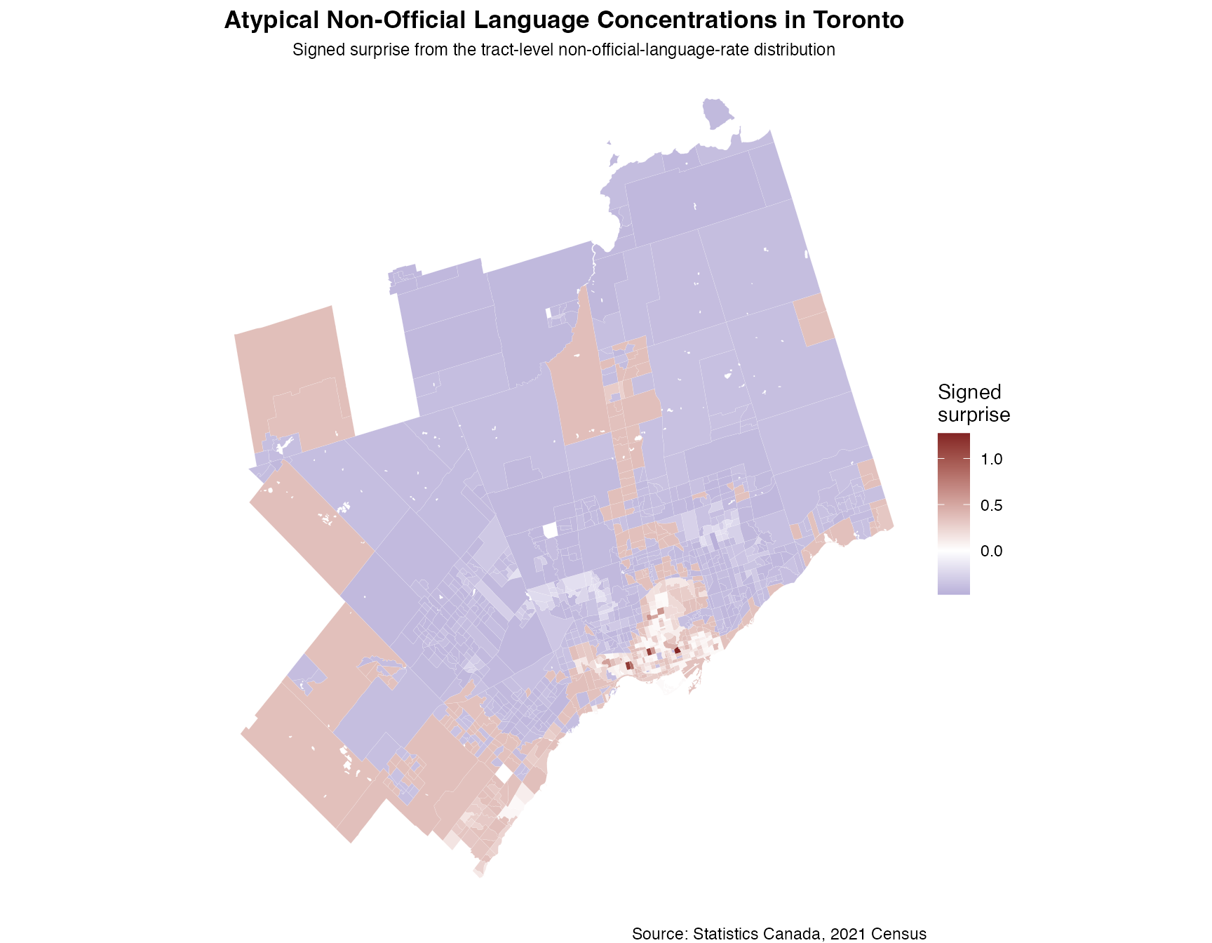
Identify areas with high model-conditional surprise for non-official language speakers at home.
# Get language data for Toronto CMA
# v_CA21_1144: Total - Knowledge of official languages
# v_CA21_1153: Neither English nor French

language_data <- get_census(
  dataset = "CA21",
  regions = list(CMA = "35535"),  # Toronto CMA
  vectors = c(
    total_pop = "v_CA21_1144",  # Total population
    no_official = "v_CA21_1153"   # Neither official language
  ),
  level = "CT",
  geo_format = "sf",
  labels = "short",
  quiet = TRUE
)

language_data <- language_data %>%
  filter(!is.na(total_pop) & !is.na(no_official)) %>%
  filter(total_pop > 100) %>%
  mutate(no_official_rate = no_official / total_pop)
# Compute surprise on the non-official-language-rate distribution.
lang_surprise <- surprise(
  language_data,
  observed = no_official_rate,
  models = c("uniform", "gaussian", "sampled")
)

language_data$signed_surprise <- get_surprise(lang_surprise, "signed")

# Plot Toronto
ggplot(language_data) +
  geom_sf(aes(fill = signed_surprise), color = "white", linewidth = 0.02) +
  scale_fill_surprise_diverging(name = "Signed\nsurprise") +
  labs(
    title = "Atypical Non-Official Language Concentrations in Toronto",
    subtitle = "Signed surprise from the tract-level non-official-language-rate distribution",
    caption = "Source: Statistics Canada, 2021 Census"
  ) +
  theme_void() +
  theme(
    legend.position = "right",
    plot.title = element_text(hjust = 0.5, face = "bold"),
    plot.subtitle = element_text(hjust = 0.5, size = 9)
  )
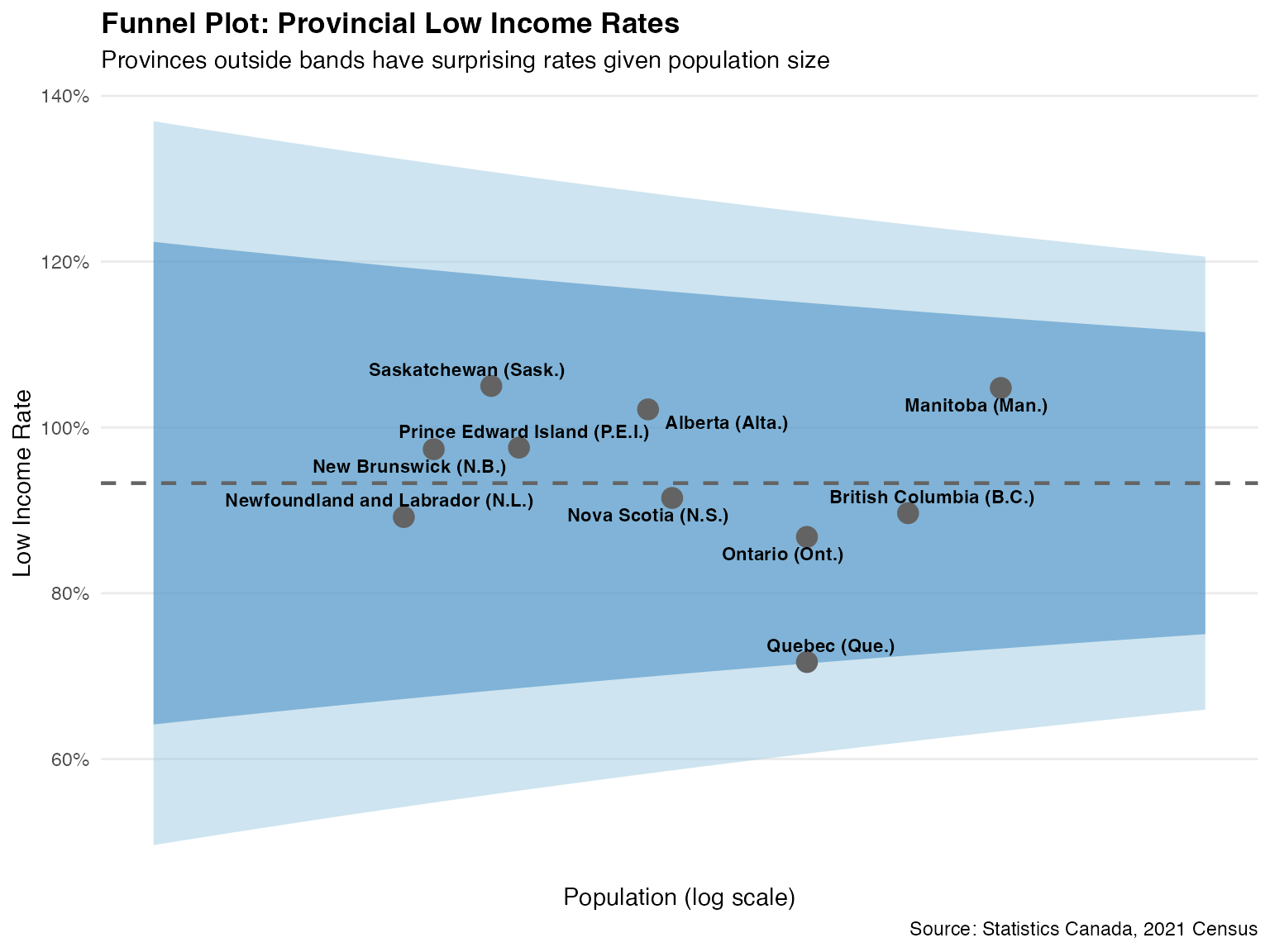
Example 4: Provincial Comparison with Funnel Plot
Compare provinces using a funnel plot to account for population size variation.
# Get provincial data
provincial_data <- get_census(
  dataset = "CA21",
  regions = list(C = "01"),
  vectors = c(
    total_pop = "v_CA21_1085",  # Total for low income
    low_income = "v_CA21_1090"   # In low income
  ),
  level = "PR",
  geo_format = NA,
  labels = "short",
  quiet = TRUE
)

provincial_data <- provincial_data %>%
  filter(!is.na(total_pop) & total_pop > 0)

# Compute funnel data for points
funnel_df <- compute_funnel_data(
  observed = provincial_data$low_income,
  sample_size = provincial_data$total_pop,
  type = "count",
  limits = c(2, 3)
)
funnel_df$province <- provincial_data$`Region Name`
funnel_df$rate <- funnel_df$observed / funnel_df$sample_size

# National rate
national_rate <- sum(provincial_data$low_income) / sum(provincial_data$total_pop)

# Create continuous funnel bands
n_range <- range(provincial_data$total_pop)
n_seq <- exp(seq(log(n_range[1] * 0.8), log(n_range[2] * 1.2), length.out = 200))
se_seq <- sqrt(national_rate * (1 - national_rate) / n_seq)

funnel_bands <- data.frame(
  n = n_seq,
  rate = national_rate,
  lower_2sd = national_rate - 2 * se_seq,
  upper_2sd = national_rate + 2 * se_seq,
  lower_3sd = national_rate - 3 * se_seq,
  upper_3sd = national_rate + 3 * se_seq
)

# Create funnel plot
ggplot() +
  # 3 SD band (outer)
  geom_ribbon(
    data = funnel_bands,
    aes(x = n, ymin = lower_3sd, ymax = upper_3sd),
    fill = "#9ecae1", alpha = 0.5
  ) +
  # 2 SD band (inner)
  geom_ribbon(
    data = funnel_bands,
    aes(x = n, ymin = lower_2sd, ymax = upper_2sd),
    fill = "#3182bd", alpha = 0.5
  ) +
  # National average line
  geom_hline(
    yintercept = national_rate,
    linetype = "dashed", color = "#636363", linewidth = 0.8
  ) +
  # Points
  geom_point(
    data = funnel_df,
    aes(x = sample_size, y = rate, color = abs(z_score) > 2),
    size = 4
  ) +
  # Labels
  ggrepel::geom_text_repel(
    data = funnel_df,
    aes(x = sample_size, y = rate, label = province),
    size = 3, fontface = "bold",
    max.overlaps = 15,
    segment.color = "gray60"
  ) +
  scale_color_manual(
    values = c("FALSE" = "#636363", "TRUE" = "#e6550d"),
    guide = "none"
  ) +
  scale_x_log10(
    labels = scales::comma,
    breaks = c(1e4, 1e5, 1e6, 1e7)
  ) +
  scale_y_continuous(labels = scales::percent) +
  labs(
    title = "Funnel Plot: Provincial Low Income Rates",
    subtitle = "Provinces outside bands have surprising rates given population size",
    x = "Population (log scale)",
    y = "Low Income Rate",
    caption = "Source: Statistics Canada, 2021 Census"
  ) +
  theme_minimal() +
  theme(
    plot.title = element_text(face = "bold"),
    panel.grid.minor = element_blank()
  )
Example 5: Comparing Census Years
Compare surprise patterns between 2016 and 2021 Census at the provincial level.
# Get provincial data for 2016 and 2021
# Note: Variable IDs differ between Census years

# 2021 data
prov_2021 <- get_census(
  dataset = "CA21",
  regions = list(C = "01"),
  vectors = c(total_pop = "v_CA21_1085", low_income = "v_CA21_1090"),
  level = "PR",
  geo_format = NA,
  labels = "short",
  quiet = TRUE
)
prov_2021 <- prov_2021[!is.na(prov_2021$total_pop) & prov_2021$total_pop > 0, ]
prov_2021$low_income_rate <- prov_2021$low_income / prov_2021$total_pop
prov_2021$census_year <- 2021

# 2016 data (different vector IDs for same concept)
prov_2016 <- get_census(
  dataset = "CA16",
  regions = list(C = "01"),
  vectors = c(total_pop = "v_CA16_2540", low_income = "v_CA16_2555"),
  level = "PR",
  geo_format = NA,
  labels = "short",
  quiet = TRUE
)
prov_2016 <- prov_2016[!is.na(prov_2016$total_pop) & prov_2016$total_pop > 0, ]
prov_2016$low_income_rate <- prov_2016$low_income / prov_2016$total_pop
prov_2016$census_year <- 2016

# Compute surprise for each year's provincial low-income-rate distribution
surprise_2021 <- surprise(
  prov_2021,
  observed = low_income_rate,
  models = c("uniform", "gaussian", "sampled")
)
prov_2021$signed_surprise <- get_surprise(surprise_2021, "signed")

surprise_2016 <- surprise(
  prov_2016,
  observed = low_income_rate,
  models = c("uniform", "gaussian", "sampled")
)
prov_2016$signed_surprise <- get_surprise(surprise_2016, "signed")

# Compare changes
comparison <- merge(
  prov_2016[, c("GeoUID", "Region Name", "signed_surprise")],
  prov_2021[, c("GeoUID", "signed_surprise")],
  by = "GeoUID",
  suffixes = c("_2016", "_2021")
)
comparison$change <- comparison$signed_surprise_2021 - comparison$signed_surprise_2016
print(comparison[order(abs(comparison$change), decreasing = TRUE), ])
#>    GeoUID               Region Name signed_surprise_2016 signed_surprise_2021
#> 4      13             New Brunswick            -1.584420           0.17272244
#> 10     59          British Columbia             1.584569          -0.17225122
#> 2      11      Prince Edward Island            -1.584443           0.17185215
#> 6      35                   Ontario             1.584877          -0.13850732
#> 7      46                  Manitoba            -1.584409           0.11617269
#> 8      47              Saskatchewan            -1.584411           0.11230080
#> 5      24                    Quebec             1.584706          -0.09813818
#> 9      48                   Alberta             1.584557           0.14575026
#> 1      10 Newfoundland and Labrador            -1.584428          -0.16841634
#> 3      12               Nova Scotia            -1.584414          -0.18158511
#>       change
#> 4   1.757143
#> 10 -1.756820
#> 2   1.756295
#> 6  -1.723384
#> 7   1.700582
#> 8   1.696712
#> 5  -1.682844
#> 9  -1.438807
#> 1   1.416012
#> 3   1.402828
Note: This example is not evaluated because it requires multiple API calls. Run locally with your CensusMapper API key.
Example 6: Custom Model Space for Census Data
For Census data, create a custom model space that matches the quantity being modeled. Here the observed values are home-ownership rates, so the models are rate-distribution models rather than population-baseline count models.
# Using the Vancouver housing data
# Create a custom model space

# Create custom model space for rates
housing_models <- model_space(
  bs_model_gaussian(),
  bs_model_sampled()
)

print(housing_models)
#> <bs_model_space>
#>   Models: 2
#>    1. Gaussian (prior: 0.5)
#>    2. Sampled (KDE) (prior: 0.5)

# Use surprise() with custom model space
custom_result <- surprise(
  housing_data,
  observed = owner_rate,
  models = housing_models
)

housing_data$custom_surprise <- get_surprise(custom_result, "signed")

# Summary statistics
cat("Custom model surprise summary:\n")
#> Custom model surprise summary:
summary(housing_data$custom_surprise)
#>       Min.    1st Qu.     Median       Mean    3rd Qu.       Max.
#> -0.4210060 -0.0035322  0.0002741 -0.0028656  0.0152084  0.0805043
Interpreting Surprise Values
Understanding what surprise values mean is crucial for proper interpretation:
| Surprise Magnitude | Interpretation | Meaning |
|---|---|---|
| < 0.1 | Trivial | Little update from prior to posterior model probabilities |
| 0.1 - 0.3 | Minor | Small model update |
| 0.3 - 0.5 | Moderate | Noticeable model update |
| 0.5 - 1.0 | Substantial | Strong model update |
| > 1.0 | High | Very strong model update under the chosen model space |
Key insight: Surprise measures how much the data discriminates between models, not just how far a rate is from average. A region with an unusual rate may show low surprise if all models assign similar likelihood to it. A region with a rate near the average can still show surprise if it falls in a part of the distribution where the chosen models disagree. Use the funnel plot separately to understand whether population size makes a rate estimate unusually reliable or noisy.
# Categorize regions by surprise level
income_data <- income_data %>%
  mutate(
    surprise_category = cut(
      abs(signed_surprise),
      breaks = c(0, 0.1, 0.3, 0.5, 1.0, Inf),
      labels = c("Trivial", "Minor", "Moderate", "Substantial", "High"),
      include.lowest = TRUE
    )
  )

# Summary by category
cat("Census Divisions by surprise level:\n")
#> Census Divisions by surprise level:
print(table(income_data$surprise_category))
#>
#>     Trivial       Minor    Moderate Substantial        High
#>         249          10           7           8           2
Session Info
sessionInfo()
#> R version 4.5.0 (2025-04-11)
#> Platform: aarch64-apple-darwin20
#> Running under: macOS Sequoia 15.4.1
#>
#> Matrix products: default
#> BLAS:   /Library/Frameworks/R.framework/Versions/4.5-arm64/Resources/lib/libRblas.0.dylib
#> LAPACK: /Library/Frameworks/R.framework/Versions/4.5-arm64/Resources/lib/libRlapack.dylib;  LAPACK version 3.12.1
#>
#> locale:
#> [1] C.UTF-8/C.UTF-8/C.UTF-8/C/C.UTF-8/C.UTF-8
#>
#> time zone: America/Los_Angeles
#> tzcode source: internal
#>
#> attached base packages:
#> [1] stats     graphics  grDevices utils     datasets  methods   base
#>
#> other attached packages:
#> [1] dplyr_1.1.4             ggplot2_4.0.1           sf_1.0-23
#> [4] cancensus_0.5.7         bayesiansurpriser_0.1.0
#>
#> loaded via a namespace (and not attached):
#>  [1] sass_0.4.10        generics_0.1.4     class_7.3-23       KernSmooth_2.23-26
#>  [5] hms_1.1.4          digest_0.6.39      magrittr_2.0.4     evaluate_1.0.4
#>  [9] grid_4.5.0         RColorBrewer_1.1-3 fastmap_1.2.0      jsonlite_2.0.0
#> [13] ggrepel_0.9.6      e1071_1.7-17       DBI_1.2.3          httr_1.4.7
#> [17] scales_1.4.0       textshaping_1.0.1  jquerylib_0.1.4    cli_3.6.5
#> [21] crayon_1.5.3       rlang_1.1.7        units_1.0-0        bit64_4.6.0-1
#> [25] withr_3.0.2        cachem_1.1.0       yaml_2.3.10        parallel_4.5.0
#> [29] tools_4.5.0        tzdb_0.5.0         geojsonsf_2.0.3    curl_7.0.0
#> [33] vctrs_0.7.0        R6_2.6.1           proxy_0.4-28       lifecycle_1.0.5
#> [37] classInt_0.4-11    bit_4.6.0          fs_1.6.6           htmlwidgets_1.6.4
#> [41] vroom_1.6.7        MASS_7.3-65        ragg_1.4.0         pkgconfig_2.0.3
#> [45] desc_1.4.3         pkgdown_2.1.3      pillar_1.11.1      bslib_0.9.0
#> [49] gtable_0.3.6       glue_1.8.0         Rcpp_1.1.0         systemfonts_1.2.3
#> [53] xfun_0.52          tibble_3.3.1       tidyselect_1.2.1   knitr_1.50
#> [57] farver_2.1.2       htmltools_0.5.8.1  labeling_0.4.3     rmarkdown_2.29
#> [61] readr_2.1.6        compiler_4.5.0     S7_0.2.1