Bayesian Surprise with US Census Data (tidycensus)
Source:vignettes/tidycensus-workflow.Rmd
tidycensus-workflow.RmdIntroduction
This vignette demonstrates how to use the
bayesiansurpriser package with US Census data accessed
through the tidycensus package.
Important: Bayesian Surprise is conditional on the model space you choose. For count/exposure data, population size can strongly affect the posterior model update because sampling variation is much smaller in large populations than in small populations. Compare results against the raw rate and a funnel plot before interpreting a map.
ACS estimates are not literal event counts from a simple random experiment. In the examples below, the surprise maps model poverty rates directly using distributional models. The funnel plot remains useful as a separate diagnostic for whether extreme rates are also credible given different population sizes.
When to Use Bayesian Surprise
The examples below are most interpretable for:
- State-level comparisons where populations are more similar
- Counties within a single state (similar geographic scale)
- Census tracts within a metro area (similar population sizes)
- Any dataset where populations do not span orders of magnitude
Prerequisites
You’ll need a Census API key from https://api.census.gov/data/key_signup.html
library(bayesiansurpriser)
library(tidycensus)
library(tigris)
library(sf)
library(ggplot2)
library(dplyr)

# Set your Census API key (do this once)
# census_api_key("YOUR_KEY_HERE", install = TRUE)
Example 1: State-Level Poverty Analysis
State-level analysis is a useful starting point because the number of units is small enough to inspect manually and the rate distribution is easy to compare against a companion funnel plot.
# Get state-level poverty data
state_poverty <- get_acs(
geography = "state",
variables = c(
total_pop = "B17001_001",
in_poverty = "B17001_002"
),
year = 2022,
survey = "acs5",
geometry = TRUE,
output = "wide"
)
#> | | | 0% | | | 1% | |= | 1% | |= | 2% | |== | 3% | |=== | 4% | |=== | 5% | |==== | 5% | |==== | 6% | |===== | 6% | |===== | 7% | |===== | 8% | |====== | 8% | |====== | 9% | |======= | 10% | |======= | 11% | |======== | 11% | |======== | 12% | |========= | 13% | |========= | 14% | |========== | 14% | |========== | 15% | |=========== | 15% | |=========== | 16% | |============ | 17% | |============ | 18% | |============= | 18% | |============= | 19% | |============== | 20% | |============== | 21% | |=============== | 21% | |=============== | 22% | |================ | 23% | |================= | 24% | |================= | 25% | |================== | 25% | |================== | 26% | |=================== | 27% | |=================== | 28% | |==================== | 28% | |==================== | 29% | |===================== | 30% | |===================== | 31% | |====================== | 31% | |====================== | 32% | |======================= | 32% | |======================= | 33% | |======================== | 34% | |======================== | 35% | |========================= | 35% | |========================= | 36% | |========================== | 37% | |========================== | 38% | |=========================== | 38% | |=========================== | 39% | |============================ | 40% | |============================= | 41% | |============================= | 42% | |============================== | 42% | |============================== | 43% | |=============================== | 44% | |=============================== | 45% | |================================ | 45% | |================================ | 46% | |================================= | 47% | |================================= | 48% | |================================== | 48% | |================================== | 49% | |=================================== | 49% | |=================================== | 50% | |==================================== | 51% | |==================================== | 52% | |===================================== | 52% | |===================================== | 53% | |====================================== | 54% | |====================================== | 55% | |======================================= | 55% | |======================================= | 56% | |======================================== | 57% | |========================================= | 58% | |========================================= | 59% | |========================================== | 59% | |========================================== | 60% | |=========================================== | 61% | |=========================================== | 62% | |============================================ | 62% | |============================================ | 63% | |============================================= | 64% | |============================================= | 65% | |============================================== | 65% | |============================================== | 66% | |=============================================== | 66% | |=============================================== | 67% | |================================================ | 68% | |================================================ | 69% | |================================================= | 69% | |================================================= | 70% | |================================================= | 71% | |================================================== | 71% | |================================================== | 72% | |=================================================== | 73% | |=================================================== | 74% | |==================================================== | 74% | |==================================================== | 75% | |===================================================== | 75% | |===================================================== | 76% | |====================================================== | 77% | |====================================================== | 78% | |======================================================= | 78% | |======================================================= | 79% | |======================================================== | 80% | |======================================================== | 81% | |========================================================= | 81% | |========================================================= | 82% | |========================================================== | 83% | |=========================================================== | 84% | |=========================================================== | 85% | |============================================================ | 85% | |============================================================ | 86% | |============================================================= | 87% | |============================================================= | 88% | |============================================================== | 88% | |============================================================== | 89% | |=============================================================== | 90% | |=============================================================== | 91% | |================================================================ | 91% | |================================================================ | 92% | |================================================================= | 92% | |================================================================= | 93% | |================================================================== | 94% | |================================================================== | 95% | |=================================================================== | 95% | |=================================================================== | 96% | |==================================================================== | 97% | |==================================================================== | 98% | |===================================================================== | 98% | |===================================================================== | 99% | |======================================================================| 100%
state_poverty <- state_poverty %>%
filter(!is.na(in_povertyE) & !is.na(total_popE)) %>%
filter(total_popE > 0) %>%
mutate(poverty_rate = in_povertyE / total_popE)
# Compute surprise on the poverty-rate distribution.
# This asks which state rates are unusual relative to the cross-state pattern.
state_surprise <- surprise(
state_poverty,
observed = poverty_rate,
models = c("uniform", "gaussian", "sampled")
)
# View results
cat("Surprise value range:", round(range(state_surprise$surprise), 4), "\n")
#> Surprise value range: 0.1718 0.5959
# States with positive signed surprise
state_surprise %>%
st_drop_geometry() %>%
filter(signed_surprise > 0) %>%
arrange(desc(surprise)) %>%
select(NAME, poverty_rate, total_popE, surprise, signed_surprise) %>%
head(10)
#> Bayesian Surprise Map
#> =====================
#>
#> NAME poverty_rate total_popE surprise signed_surprise
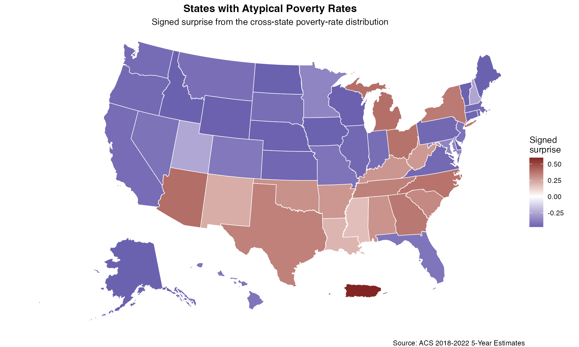
#> 1 Puerto Rico 0.4219536 3242916 0.5959455 0.5959455
#> 2 Arizona 0.1306505 7017776 0.3928159 0.3928159
#> 3 Michigan 0.1313491 9845242 0.3891079 0.3891079
#> 4 Ohio 0.1330563 11472644 0.3794113 0.3794113
#> 5 North Carolina 0.1332611 10186155 0.3781859 0.3781859
#> 6 Georgia 0.1353006 10462430 0.3653745 0.3653745
#> 7 New York 0.1360694 19516967 0.3603671 0.3603671
#> 8 Texas 0.1394442 28615931 0.3386187 0.3386187
#> 9 Tennessee 0.1395926 6759549 0.3377102 0.3377102
#> 10 South Carolina 0.1435029 5002332 0.3170755 0.3170755
# States with negative signed surprise
state_surprise %>%
  st_drop_geometry() %>%
  filter(signed_surprise < 0) %>%
  arrange(desc(surprise)) %>%
  select(NAME, poverty_rate, total_popE, surprise, signed_surprise) %>%
  head(10)
#> Bayesian Surprise Map
#> =====================
#>
#>            NAME poverty_rate total_popE  surprise signed_surprise
#> 1  North Dakota    0.1076353     750776 0.4653261      -0.4653261
#> 2       Wyoming    0.1066007     564105 0.4651773      -0.4651773
#> 3     Wisconsin    0.1065024    5743164 0.4651136      -0.4651136
#> 4         Maine    0.1094367    1329454 0.4636159      -0.4636159
#> 5        Alaska    0.1048763     717293 0.4629998      -0.4629998
#> 6         Idaho    0.1101173    1805238 0.4624379      -0.4624379
#> 7       Vermont    0.1042702     620877 0.4615756      -0.4615756
#> 8      Nebraska    0.1039844    1908613 0.4607026      -0.4607026
#> 9          Iowa    0.1110849    3088999 0.4603493      -0.4603493
#> 10     Delaware    0.1112298     969075 0.4600026      -0.4600026
Visualize State-Level Results
# Shift AK/HI for visualization
state_surprise_shifted <- state_surprise %>%
  shift_geometry()

ggplot(state_surprise_shifted) +
  geom_sf(aes(fill = signed_surprise), color = "white", linewidth = 0.3) +
  scale_fill_surprise_diverging(name = "Signed\nsurprise") +
  labs(
    title = "States with Atypical Poverty Rates",
    subtitle = "Signed surprise from the cross-state poverty-rate distribution",
    caption = "Source: ACS 2018-2022 5-Year Estimates"
  ) +
  theme_void() +
  theme(
    legend.position = "right",
    plot.title = element_text(hjust = 0.5, face = "bold"),
    plot.subtitle = element_text(hjust = 0.5)
  )
Example 2: Funnel Plot Visualization
Funnel plots show how rates vary with population size and provide context for sampling variation.
library(ggrepel)

# Compute funnel data
funnel_df <- compute_funnel_data(
  observed = state_poverty$in_povertyE,
  sample_size = state_poverty$total_popE,
  type = "count",
  limits = c(2, 3)
)
funnel_df$state <- state_poverty$NAME
funnel_df$rate <- funnel_df$observed / funnel_df$sample_size

# National rate
national_rate <- sum(state_poverty$in_povertyE) / sum(state_poverty$total_popE)

# Create funnel bands
n_range <- range(state_poverty$total_popE)
n_seq <- exp(seq(log(n_range[1] * 0.8), log(n_range[2] * 1.2), length.out = 200))
se_seq <- sqrt(national_rate * (1 - national_rate) / n_seq)

funnel_bands <- data.frame(
  n = n_seq,
  lower_2sd = national_rate - 2 * se_seq,
  upper_2sd = national_rate + 2 * se_seq,
  lower_3sd = national_rate - 3 * se_seq,
  upper_3sd = national_rate + 3 * se_seq
)

# Plot
ggplot() +
  geom_ribbon(
    data = funnel_bands,
    aes(x = n, ymin = lower_3sd, ymax = upper_3sd),
    fill = "#9ecae1", alpha = 0.5
  ) +
  geom_ribbon(
    data = funnel_bands,
    aes(x = n, ymin = lower_2sd, ymax = upper_2sd),
    fill = "#3182bd", alpha = 0.5
  ) +
  geom_hline(yintercept = national_rate, linetype = "dashed", color = "#636363") +
  geom_point(
    data = funnel_df,
    aes(x = sample_size, y = rate, color = abs(z_score) > 2),
    size = 3
  ) +
  geom_text_repel(
    data = funnel_df %>% filter(abs(z_score) > 2),
    aes(x = sample_size, y = rate, label = state),
    size = 3, fontface = "bold"
  ) +
  scale_color_manual(values = c("FALSE" = "#636363", "TRUE" = "#e6550d"), guide = "none") +
  scale_x_log10(labels = scales::comma) +
  scale_y_continuous(labels = scales::percent) +
  labs(
    title = "Funnel Plot: State Poverty Rates",
    subtitle = "States outside bands have rates that are unusual for their population size",
    x = "Population (log scale)",
    y = "Poverty Rate"
  ) +
  theme_minimal()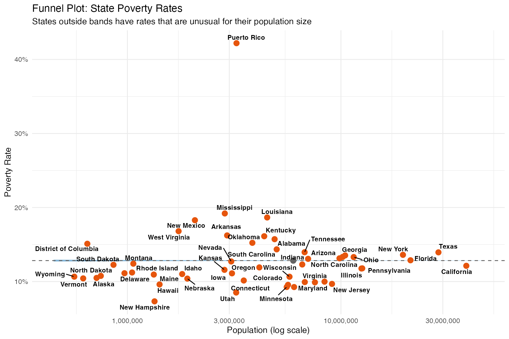
Why doesn’t this look like a funnel? State populations only span ~2 orders of magnitude (580K to 39M). At these large sample sizes, standard errors are tiny and nearly identical, so the control bands appear as horizontal lines. We’re seeing only the narrow right edge of what would be a funnel.
County-Level Funnel (Classic Shape)
To see a true funnel, we need data spanning many orders of magnitude. US counties range from ~50 to ~10 million people, making the changing uncertainty bands easy to see.
# Get all county poverty data (no geometry needed for funnel plot)
county_poverty_all <- get_acs(
  geography = "county",
  variables = c(
    total_pop = "B17001_001",
    in_poverty = "B17001_002"
  ),
  year = 2022,
  survey = "acs5",
  output = "wide"
) %>%
  filter(!is.na(in_povertyE) & !is.na(total_popE)) %>%
  filter(total_popE > 0) %>%
  mutate(poverty_rate = in_povertyE / total_popE)

cat("County population range:", format(range(county_poverty_all$total_popE), big.mark = ","), "\n")
#> County population range:        47 9,782,602
cat("Number of counties:", nrow(county_poverty_all), "\n")
#> Number of counties: 3222

# National rate from county data
national_rate_county <- sum(county_poverty_all$in_povertyE) / sum(county_poverty_all$total_popE)

# Compute funnel data
county_funnel <- compute_funnel_data(
  observed = county_poverty_all$in_povertyE,
  sample_size = county_poverty_all$total_popE,
  type = "count",
  limits = c(2, 3)
)
county_funnel$name <- county_poverty_all$NAME
county_funnel$rate <- county_funnel$observed / county_funnel$sample_size

# Create funnel bands across full range
n_range_county <- range(county_poverty_all$total_popE)
n_seq_county <- exp(seq(log(n_range_county[1] * 0.8), log(n_range_county[2] * 1.2), length.out = 300))
se_seq_county <- sqrt(national_rate_county * (1 - national_rate_county) / n_seq_county)

county_bands <- data.frame(
  n = n_seq_county,
  lower_2sd = national_rate_county - 2 * se_seq_county,
  upper_2sd = national_rate_county + 2 * se_seq_county,
  lower_3sd = national_rate_county - 3 * se_seq_county,
  upper_3sd = national_rate_county + 3 * se_seq_county
)

# Identify extreme outliers for labeling
extreme_counties <- county_funnel %>%
  filter(abs(z_score) > 4) %>%
  arrange(desc(abs(z_score))) %>%
  head(15)

# Plot
ggplot() +
  geom_ribbon(
    data = county_bands,
    aes(x = n, ymin = pmax(lower_3sd, 0), ymax = pmin(upper_3sd, 1)),
    fill = "#9ecae1", alpha = 0.5
  ) +
  geom_ribbon(
    data = county_bands,
    aes(x = n, ymin = pmax(lower_2sd, 0), ymax = pmin(upper_2sd, 1)),
    fill = "#3182bd", alpha = 0.5
  ) +
  geom_hline(yintercept = national_rate_county, linetype = "dashed", color = "#636363") +
  geom_point(
    data = county_funnel,
    aes(x = sample_size, y = rate, color = abs(z_score) > 3),
    size = 1, alpha = 0.6
  ) +
  geom_text_repel(
    data = extreme_counties,
    aes(x = sample_size, y = rate, label = name),
    size = 2.5, fontface = "bold", max.overlaps = 20
  ) +
  scale_color_manual(values = c("FALSE" = "#636363", "TRUE" = "#e6550d"), guide = "none") +
  scale_x_log10(labels = scales::comma) +
  scale_y_continuous(labels = scales::percent, limits = c(0, 0.7)) +
  labs(
    title = "Funnel Plot: County Poverty Rates (All US Counties)",
    subtitle = "Classic funnel shape: wide bands for small populations, narrow for large",
    x = "Population (log scale)",
    y = "Poverty Rate",
    caption = "Orange = |z| > 3 | Labeled = |z| > 4"
  ) +
  theme_minimal()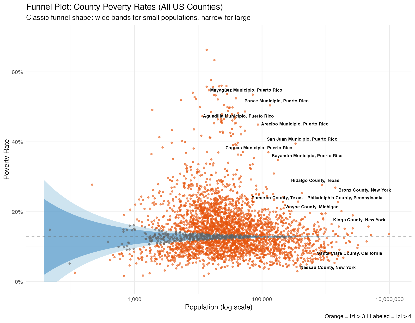
Key insight: Small counties (left side) have wide control bands - rates from 5% to 25% are all “expected” given sampling variation. Large counties (right side) have narrow bands, so smaller deviations from ~13% can strongly update the model posterior.
This explains why a funnel diagnostic can differ from a rate map: - A small county with an extreme rate may still be plausible under a sampling-variation model. - A large county with a modest rate difference can still be unusual because its sampling variation is small.
Example 3: Tract-Level Analysis (Same-Scale Comparison)
Census tracts within a metro area have similar populations (~2,000-8,000), making the model comparison easier to interpret than an all-county national map.
# Get tract-level data for Cook County (Chicago)
chicago_tracts <- get_acs(
geography = "tract",
state = "IL",
county = "Cook",
variables = c(
total_pop = "B17001_001",
in_poverty = "B17001_002"
),
year = 2022,
survey = "acs5",
geometry = TRUE,
output = "wide"
)
#> | | | 0% | |= | 1% | |== | 2% | |== | 3% | |=== | 4% | |==== | 5% | |===== | 7% | |===== | 8% | |======= | 10% | |======== | 11% | |======== | 12% | |========= | 13% | |========== | 14% | |=========== | 15% | |=========== | 16% | |============ | 17% | |============= | 19% | |============== | 20% | |=============== | 21% | |=============== | 22% | |================ | 23% | |================= | 24% | |================== | 25% | |================== | 26% | |=================== | 27% | |==================== | 28% | |===================== | 30% | |===================== | 31% | |====================== | 32% | |======================= | 33% | |======================== | 34% | |======================== | 35% | |========================= | 36% | |========================== | 37% | |=========================== | 38% | |============================ | 39% | |============================ | 40% | |============================= | 42% | |============================== | 43% | |=============================== | 44% | |=============================== | 45% | |================================ | 46% | |================================= | 47% | |================================== | 48% | |================================== | 49% | |=================================== | 50% | |==================================== | 51% | |===================================== | 53% | |====================================== | 54% | |====================================== | 55% | |======================================= | 56% | |======================================== | 57% | |========================================= | 58% | |========================================= | 59% | |========================================== | 60% | |=========================================== | 61% | |============================================ | 62% | |============================================ | 63% | |============================================= | 65% | |============================================== | 66% | |=============================================== | 67% | |=============================================== | 68% | |================================================ | 69% | |================================================= | 70% | |================================================== | 71% | |=================================================== | 72% | |=================================================== | 73% | |==================================================== | 74% | |===================================================== | 76% | |====================================================== | 77% | |====================================================== | 78% | |======================================================= | 79% | |======================================================== | 80% | |========================================================= | 81% | |========================================================= | 82% | |========================================================== | 83% | |=========================================================== | 84% | |============================================================ | 85% | |============================================================= | 86% | |============================================================= | 88% | |============================================================== | 89% | |=============================================================== | 90% | |================================================================ | 91% | |================================================================ | 92% | |================================================================= | 93% | |================================================================== | 94% | |=================================================================== | 95% | |=================================================================== | 96% | |==================================================================== | 97% | |===================================================================== | 99% | |======================================================================| 100%
chicago_tracts <- chicago_tracts %>%
filter(!is.na(in_povertyE) & !is.na(total_popE)) %>%
filter(total_popE > 100) %>%
mutate(poverty_rate = in_povertyE / total_popE)
cat("Population range:", range(chicago_tracts$total_popE), "\n")
#> Population range: 306 12213
cat("Number of tracts:", nrow(chicago_tracts), "\n")
#> Number of tracts: 1328
# Compute surprise on the poverty-rate distribution.
# The funnel plot above is the companion check for sample-size reliability.
chicago_surprise <- surprise(
chicago_tracts,
observed = poverty_rate,
models = c("uniform", "gaussian", "sampled")
)
# Plot
ggplot(chicago_surprise) +
geom_sf(aes(fill = surprise), color = NA) +
scale_fill_surprise(option = "magma", name = "Surprise\n(bits)") +
labs(
title = "Atypical Poverty Rates in Cook County, IL",
subtitle = "Census tracts far from the countywide poverty-rate distribution",
caption = "Source: ACS 2018-2022 5-Year Estimates"
) +
theme_void()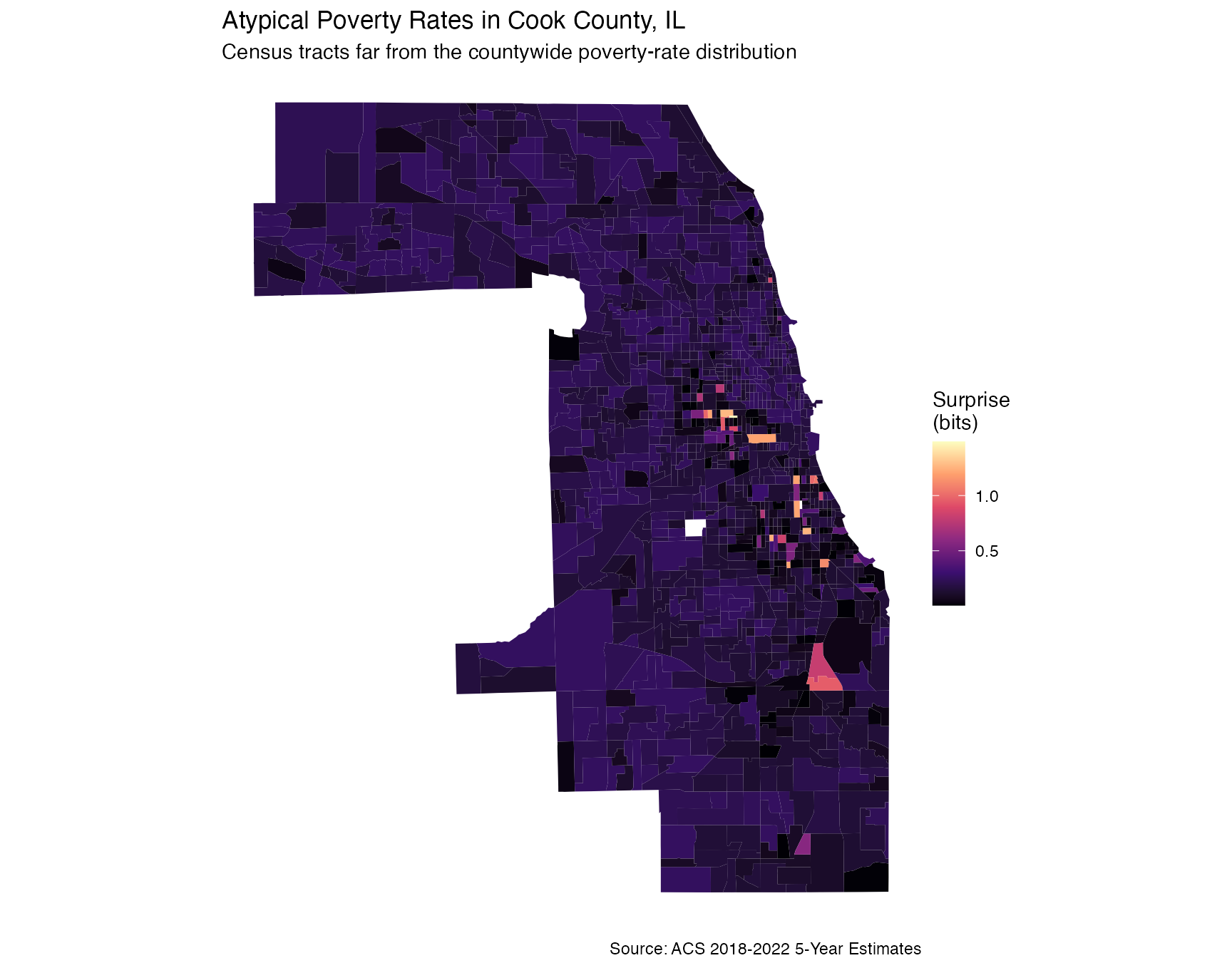
# Largest signed surprise values under the rate-distribution model space
chicago_surprise %>%
  st_drop_geometry() %>%
  mutate(poverty_rate = in_povertyE / total_popE) %>%
  arrange(desc(abs(signed_surprise))) %>%
  select(NAME, poverty_rate, total_popE, surprise, signed_surprise) %>%
  head(10)
#> Bayesian Surprise Map
#> =====================
#>
#>                                        NAME poverty_rate total_popE surprise
#> 1  Census Tract 8369; Cook County; Illinois    0.7557673       1994 1.487703
#> 2  Census Tract 8368; Cook County; Illinois    0.6394687       2635 1.272643
#> 3  Census Tract 4008; Cook County; Illinois    0.6361994       2768 1.257259
#> 4  Census Tract 6711; Cook County; Illinois    0.6316940        915 1.239242
#> 5  Census Tract 8356; Cook County; Illinois    0.6194927        749 1.209598
#> 6  Census Tract 2603; Cook County; Illinois    0.5957333       1875 1.207327
#> 7  Census Tract 7101; Cook County; Illinois    0.5974659       1026 1.206541
#> 8  Census Tract 8429; Cook County; Illinois    0.6097637       3216 1.202876
#> 9  Census Tract 3406; Cook County; Illinois    0.5797101       1311 1.202058
#> 10 Census Tract 6915; Cook County; Illinois    0.5583113       1895 1.116026
#>    signed_surprise
#> 1         1.487703
#> 2         1.272643
#> 3         1.257259
#> 4         1.239242
#> 5         1.209598
#> 6         1.207327
#> 7         1.206541
#> 8         1.202876
#> 9         1.202058
#> 10        1.116026
Example 4: Large Counties Only
When analyzing all US counties, filtering to larger populations gives more interpretable rate-distribution results and keeps the companion funnel plot from being driven entirely by very small places.
# Get county data
county_poverty <- get_acs(
geography = "county",
variables = c(
total_pop = "B17001_001",
in_poverty = "B17001_002"
),
year = 2022,
survey = "acs5",
geometry = TRUE,
output = "wide"
) %>%
shift_geometry()
#> | | | 0% | | | 1% | |= | 1% | |= | 2% | |== | 2% | |== | 3% | |== | 4% | |=== | 4% | |=== | 5% | |==== | 5% | |==== | 6% | |===== | 6% | |===== | 7% | |===== | 8% | |====== | 8% | |====== | 9% | |======= | 9% | |======= | 10% | |======= | 11% | |======== | 11% | |======== | 12% | |========= | 12% | |========= | 13% | |========== | 14% | |========== | 15% | |=========== | 15% | |=========== | 16% | |============ | 16% | |============ | 17% | |============ | 18% | |============= | 18% | |============= | 19% | |============== | 19% | |============== | 20% | |============== | 21% | |=============== | 21% | |=============== | 22% | |================ | 22% | |================ | 23% | |================= | 24% | |================= | 25% | |================== | 25% | |================== | 26% | |=================== | 27% | |=================== | 28% | |==================== | 28% | |==================== | 29% | |===================== | 29% | |===================== | 30% | |===================== | 31% | |====================== | 31% | |====================== | 32% | |======================= | 32% | |======================= | 33% | |======================== | 34% | |======================== | 35% | |========================= | 35% | |========================= | 36% | |========================== | 37% | |========================== | 38% | |=========================== | 38% | |=========================== | 39% | |============================ | 39% | |============================ | 40% | |============================ | 41% | |============================= | 41% | |============================= | 42% | |============================== | 42% | |============================== | 43% | |============================== | 44% | |=============================== | 44% | |=============================== | 45% | |================================ | 45% | |================================ | 46% | |================================= | 47% | |================================= | 48% | |================================== | 48% | |================================== | 49% | |=================================== | 49% | |=================================== | 50% | |=================================== | 51% | |==================================== | 51% | |==================================== | 52% | |===================================== | 52% | |===================================== | 53% | |===================================== | 54% | |====================================== | 54% | |====================================== | 55% | |======================================= | 55% | |======================================= | 56% | |======================================== | 56% | |======================================== | 57% | |======================================== | 58% | |========================================= | 58% | |========================================= | 59% | |========================================== | 59% | |========================================== | 60% | |========================================== | 61% | |=========================================== | 61% | |=========================================== | 62% | |============================================ | 62% | |============================================ | 63% | |============================================ | 64% | |============================================= | 64% | |============================================= | 65% | |============================================== | 65% | |============================================== | 66% | |=============================================== | 66% | |=============================================== | 67% | |=============================================== | 68% | |================================================ | 68% | |================================================ | 69% | |================================================= | 69% | |================================================= | 70% | |================================================= | 71% | |================================================== | 71% | |================================================== | 72% | |=================================================== | 72% | |=================================================== | 73% | |=================================================== | 74% | |==================================================== | 74% | |==================================================== | 75% | |===================================================== | 75% | |===================================================== | 76% | |====================================================== | 76% | |====================================================== | 77% | |====================================================== | 78% | |======================================================= | 78% | |======================================================= | 79% | |======================================================== | 79% | |======================================================== | 80% | |======================================================== | 81% | |========================================================= | 81% | |========================================================= | 82% | |========================================================== | 82% | |========================================================== | 83% | |=========================================================== | 84% | |=========================================================== | 85% | |============================================================ | 85% | |============================================================ | 86% | |============================================================= | 86% | |============================================================= | 87% | |============================================================= | 88% | |============================================================== | 88% | |============================================================== | 89% | |=============================================================== | 89% | |=============================================================== | 90% | |=============================================================== | 91% | |================================================================ | 91% | |================================================================ | 92% | |================================================================= | 92% | |================================================================= | 93% | |================================================================== | 94% | |================================================================== | 95% | |=================================================================== | 95% | |=================================================================== | 96% | |==================================================================== | 97% | |==================================================================== | 98% | |===================================================================== | 98% | |===================================================================== | 99% | |======================================================================| 99% | |======================================================================| 100%
# Filter to counties with >100k population
large_counties <- county_poverty %>%
filter(!is.na(in_povertyE) & !is.na(total_popE)) %>%
filter(total_popE > 100000) %>%
mutate(poverty_rate = in_povertyE / total_popE)
cat("Counties with >100k population:", nrow(large_counties), "\n")
#> Counties with >100k population: 598
cat("Population range:", format(range(large_counties$total_popE), big.mark = ","), "\n")
#> Population range: 100,041 9,782,602
# Compute surprise on the county poverty-rate distribution
large_surprise <- surprise(
large_counties,
observed = poverty_rate,
models = c("uniform", "gaussian", "sampled")
)
# Largest positive signed surprise values
cat("=== POSITIVE SIGNED SURPRISE (large counties) ===\n")
#> === POSITIVE SIGNED SURPRISE (large counties) ===
large_surprise %>%
  st_drop_geometry() %>%
  filter(signed_surprise > 0) %>%
  arrange(desc(surprise)) %>%
  select(NAME, poverty_rate, total_popE, surprise, signed_surprise) %>%
  head(10)
#> Bayesian Surprise Map
#> =====================
#>
#>                               NAME poverty_rate total_popE  surprise
#> 1     Ponce Municipio, Puerto Rico    0.5042898     133340 1.2769620
#> 2  San Juan Municipio, Puerto Rico    0.3950468     335621 1.2570733
#> 3   Bayamón Municipio, Puerto Rico    0.3480910     179387 1.2407810
#> 4    Caguas Municipio, Puerto Rico    0.3702575     125961 1.2263854
#> 5  Carolina Municipio, Puerto Rico    0.3095305     153371 1.2113256
#> 6            Hidalgo County, Texas    0.2769962     863824 0.6421004
#> 7   Robeson County, North Carolina    0.2711545     114042 0.5094130
#> 8           Bronx County, New York    0.2691499    1411574 0.4716255
#> 9           Clarke County, Georgia    0.2659760     118537 0.4174260
#> 10 Pennington County, South Dakota    0.1226647     107105 0.3255835
#>    signed_surprise
#> 1        1.2769620
#> 2        1.2570733
#> 3        1.2407810
#> 4        1.2263854
#> 5        1.2113256
#> 6        0.6421004
#> 7        0.5094130
#> 8        0.4716255
#> 9        0.4174260
#> 10       0.3255835
cat("=== NEGATIVE SIGNED SURPRISE (large counties) ===\n")
#> === NEGATIVE SIGNED SURPRISE (large counties) ===
large_surprise %>%
  st_drop_geometry() %>%
  filter(signed_surprise < 0) %>%
  arrange(desc(surprise)) %>%
  select(NAME, poverty_rate, total_popE, surprise, signed_surprise) %>%
  head(10)
#> Bayesian Surprise Map
#> =====================
#>
#>                                                      NAME poverty_rate
#> 1                              Lancaster County, Nebraska    0.1180172
#> 2                             La Crosse County, Wisconsin    0.1177961
#> 3  South Central Connecticut Planning Region, Connecticut    0.1177059
#> 4                                 Tom Green County, Texas    0.1173964
#> 5                                   Pasco County, Florida    0.1181581
#> 6                                     Lee County, Florida    0.1170128
#> 7                                 Denver County, Colorado    0.1169587
#> 8                              Berks County, Pennsylvania    0.1182070
#> 9                                 Queens County, New York    0.1169338
#> 10                                    Butler County, Ohio    0.1184909
#>    total_popE  surprise signed_surprise
#> 1      309133 0.3266167      -0.3266167
#> 2      115615 0.3266163      -0.3266163
#> 3      548511 0.3266159      -0.3266159
#> 4      113564 0.3266133      -0.3266133
#> 5      560241 0.3266083      -0.3266083
#> 6      761814 0.3266077      -0.3266077
#> 7      698563 0.3266066      -0.3266066
#> 8      415500 0.3266052      -0.3266052
#> 9     2334022 0.3266047      -0.3266047
#> 10     377008 0.3265865      -0.3265865
ggplot(large_surprise) +
  geom_sf(aes(fill = signed_surprise), color = "white", linewidth = 0.1) +
  scale_fill_surprise_diverging(name = "Signed\nsurprise") +
  labs(
    title = "Atypical Poverty Rates (Counties >100k Population)",
    subtitle = "Signed surprise from the large-county poverty-rate distribution",
    caption = "Source: ACS 2018-2022 5-Year Estimates"
  ) +
  theme_void()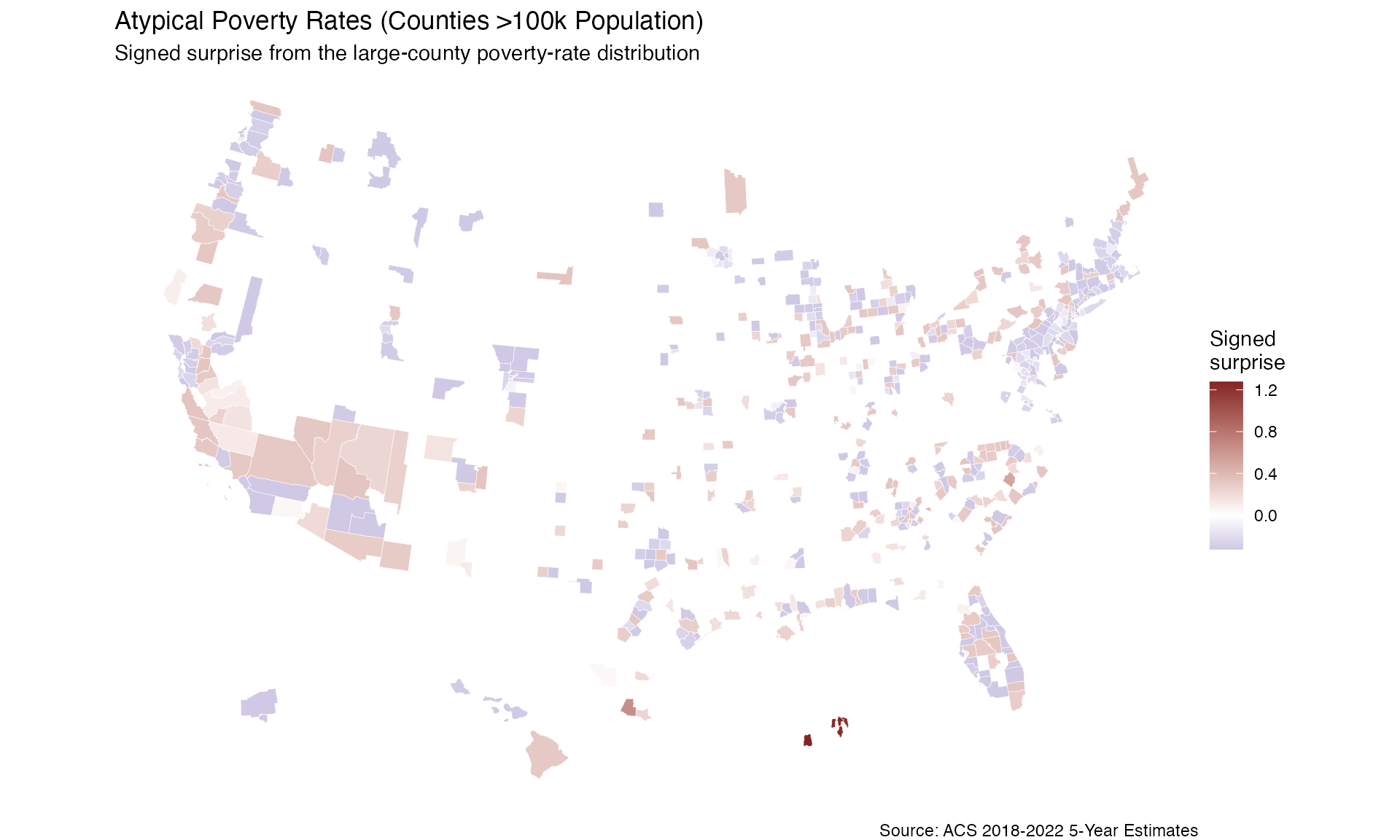
Understanding the Methodology
Why Small Regions Can Be Misleading
The funnel diagnostic accounts for sampling variation: small populations have higher expected variance in rates. This means:
- A 60% poverty rate in a county of 500 people is “expected” to vary widely
- A 60% poverty rate in a county of 500,000 people produces a much stronger model update
When populations span many orders of magnitude, use a surprise map together with the raw rate map and funnel plot so the source of the model update is visible.
Recommendations
| Data Type | Recommended Approach |
|---|---|
| States | Model the rate distribution and compare against a funnel plot |
| All counties | Filter to >50k or >100k population, or use the funnel plot as the main diagnostic |
| Counties in one state | Often easier to interpret than all counties |
| Census tracts | Model rates directly and inspect the high-surprise tracts |
| Block groups | Use with care; inspect sample-size variation |
Session Info
sessionInfo()
#> R version 4.5.0 (2025-04-11)
#> Platform: aarch64-apple-darwin20
#> Running under: macOS Sequoia 15.4.1
#>
#> Matrix products: default
#> BLAS:   /Library/Frameworks/R.framework/Versions/4.5-arm64/Resources/lib/libRblas.0.dylib
#> LAPACK: /Library/Frameworks/R.framework/Versions/4.5-arm64/Resources/lib/libRlapack.dylib;  LAPACK version 3.12.1
#>
#> locale:
#> [1] C.UTF-8/C.UTF-8/C.UTF-8/C/C.UTF-8/C.UTF-8
#>
#> time zone: America/Los_Angeles
#> tzcode source: internal
#>
#> attached base packages:
#> [1] stats     graphics  grDevices utils     datasets  methods   base
#>
#> other attached packages:
#> [1] ggrepel_0.9.6           dplyr_1.1.4             ggplot2_4.0.1
#> [4] sf_1.0-23               tigris_2.2.1            tidycensus_1.7.1
#> [7] bayesiansurpriser_0.1.0
#>
#> loaded via a namespace (and not attached):
#>  [1] tidyr_1.3.2        rappdirs_0.3.3     sass_0.4.10        generics_0.1.4
#>  [5] class_7.3-23       xml2_1.3.8         KernSmooth_2.23-26 stringi_1.8.7
#>  [9] hms_1.1.4          digest_0.6.39      magrittr_2.0.4     evaluate_1.0.4
#> [13] grid_4.5.0         RColorBrewer_1.1-3 fastmap_1.2.0      jsonlite_2.0.0
#> [17] e1071_1.7-17       DBI_1.2.3          httr_1.4.7         rvest_1.0.4
#> [21] purrr_1.2.1        viridisLite_0.4.2  scales_1.4.0       textshaping_1.0.1
#> [25] jquerylib_0.1.4    cli_3.6.5          crayon_1.5.3       rlang_1.1.7
#> [29] units_1.0-0        withr_3.0.2        cachem_1.1.0       yaml_2.3.10
#> [33] tools_4.5.0        tzdb_0.5.0         uuid_1.2-1         curl_7.0.0
#> [37] vctrs_0.7.0        R6_2.6.1           proxy_0.4-28       lifecycle_1.0.5
#> [41] classInt_0.4-11    stringr_1.6.0      fs_1.6.6           htmlwidgets_1.6.4
#> [45] MASS_7.3-65        ragg_1.4.0         pkgconfig_2.0.3    desc_1.4.3
#> [49] pkgdown_2.1.3      pillar_1.11.1      bslib_0.9.0        gtable_0.3.6
#> [53] glue_1.8.0         Rcpp_1.1.0         systemfonts_1.2.3  xfun_0.52
#> [57] tibble_3.3.1       tidyselect_1.2.1   knitr_1.50         farver_2.1.2
#> [61] htmltools_0.5.8.1  labeling_0.4.3     rmarkdown_2.29     readr_2.1.6
#> [65] compiler_4.5.0     S7_0.2.1