Introduction to bayesiansurpriser • bayesiansurpriser

Overview

The bayesiansurpriser package implements Bayesian Surprise methodology for de-biasing thematic maps and data visualizations. This technique, based on Correll & Heer’s “Surprise! Bayesian Weighting for De-Biasing Thematic Maps” (IEEE InfoVis 2016), helps identify truly surprising patterns in data by accounting for common cognitive biases.

The Problem: Cognitive Biases in Data Visualization

When viewing thematic maps or data visualizations, viewers often fall prey to three cognitive biases:

Base rate bias: Ignoring that larger populations naturally produce more events
Sampling error bias: Treating small-sample estimates as equally reliable as large-sample ones
Renormalization bias: Difficulty comparing rates across different scales

The Solution: Bayesian Surprise

Bayesian Surprise measures how much our beliefs change after observing data. Mathematically, it computes the KL-divergence between prior and posterior distributions across a space of models:

$\text{Surprise} = D_{KL}(P(M|D) \| P(M)) = \sum_i P(M_i|D) \log \frac{P(M_i|D)}{P(M_i)}$

Higher surprise indicates observations that substantially change our beliefs.

Quick Start

library(bayesiansurpriser)
#> bayesiansurpriser: Bayesian Surprise for De-Biasing Thematic Maps
#> Inspired by Correll & Heer (2017) - IEEE InfoVis
library(sf)
#> Warning: package 'sf' was built under R version 4.5.2
#> Linking to GEOS 3.13.0, GDAL 3.8.5, PROJ 9.5.1; sf_use_s2() is TRUE
library(ggplot2)
#> Warning: package 'ggplot2' was built under R version 4.5.2

Basic Usage with sf Objects

# Load North Carolina SIDS data
nc <- st_read(system.file("shape/nc.shp", package = "sf"), quiet = TRUE)

# Compute surprise: observed SIDS cases vs expected (births)
result <- surprise(nc, observed = SID74, expected = BIR74)

# View the result
print(result)
#> Bayesian Surprise Map
#> =====================
#> Models: 3 
#> Surprise range: 0.0334 to 0.6008 
#> Signed surprise range: -0.5834 to 0.6008 
#> 
#> Simple feature collection with 100 features and 16 fields
#> Geometry type: MULTIPOLYGON
#> Dimension:     XY
#> Bounding box:  xmin: -84.32385 ymin: 33.88199 xmax: -75.45698 ymax: 36.58965
#> Geodetic CRS:  NAD27
#> First 10 features:
#>     AREA PERIMETER CNTY_ CNTY_ID        NAME  FIPS FIPSNO CRESS_ID BIR74 SID74
#> 1  0.114     1.442  1825    1825        Ashe 37009  37009        5  1091     1
#> 2  0.061     1.231  1827    1827   Alleghany 37005  37005        3   487     0
#> 3  0.143     1.630  1828    1828       Surry 37171  37171       86  3188     5
#> 4  0.070     2.968  1831    1831   Currituck 37053  37053       27   508     1
#> 5  0.153     2.206  1832    1832 Northampton 37131  37131       66  1421     9
#> 6  0.097     1.670  1833    1833    Hertford 37091  37091       46  1452     7
#> 7  0.062     1.547  1834    1834      Camden 37029  37029       15   286     0
#> 8  0.091     1.284  1835    1835       Gates 37073  37073       37   420     0
#> 9  0.118     1.421  1836    1836      Warren 37185  37185       93   968     4
#> 10 0.124     1.428  1837    1837      Stokes 37169  37169       85  1612     1
#>    NWBIR74 BIR79 SID79 NWBIR79                       geometry   surprise
#> 1       10  1364     0      19 MULTIPOLYGON (((-81.47276 3... 0.19528584
#> 2       10   542     3      12 MULTIPOLYGON (((-81.23989 3... 0.11076159
#> 3      208  3616     6     260 MULTIPOLYGON (((-80.45634 3... 0.29096840
#> 4      123   830     2     145 MULTIPOLYGON (((-76.00897 3... 0.11714867
#> 5     1066  1606     3    1197 MULTIPOLYGON (((-77.21767 3... 0.57773733
#> 6      954  1838     5    1237 MULTIPOLYGON (((-76.74506 3... 0.51437420
#> 7      115   350     2     139 MULTIPOLYGON (((-76.00897 3... 0.04355317
#> 8      254   594     2     371 MULTIPOLYGON (((-76.56251 3... 0.08634903
#> 9      748  1190     2     844 MULTIPOLYGON (((-78.30876 3... 0.37427103
#> 10     160  2038     5     176 MULTIPOLYGON (((-80.02567 3... 0.31685289
#>    signed_surprise
#> 1      -0.19528584
#> 2      -0.11076159
#> 3      -0.29096840
#> 4      -0.11714867
#> 5       0.57773733
#> 6       0.51437420
#> 7      -0.04355317
#> 8      -0.08634903
#> 9       0.37427103
#> 10     -0.31685289

Plotting Results

# Plot surprise values with ggplot2
ggplot(result) +
  geom_sf(aes(fill = surprise)) +
  scale_fill_surprise() +
  labs(title = "Bayesian Surprise: NC SIDS Data (1974)")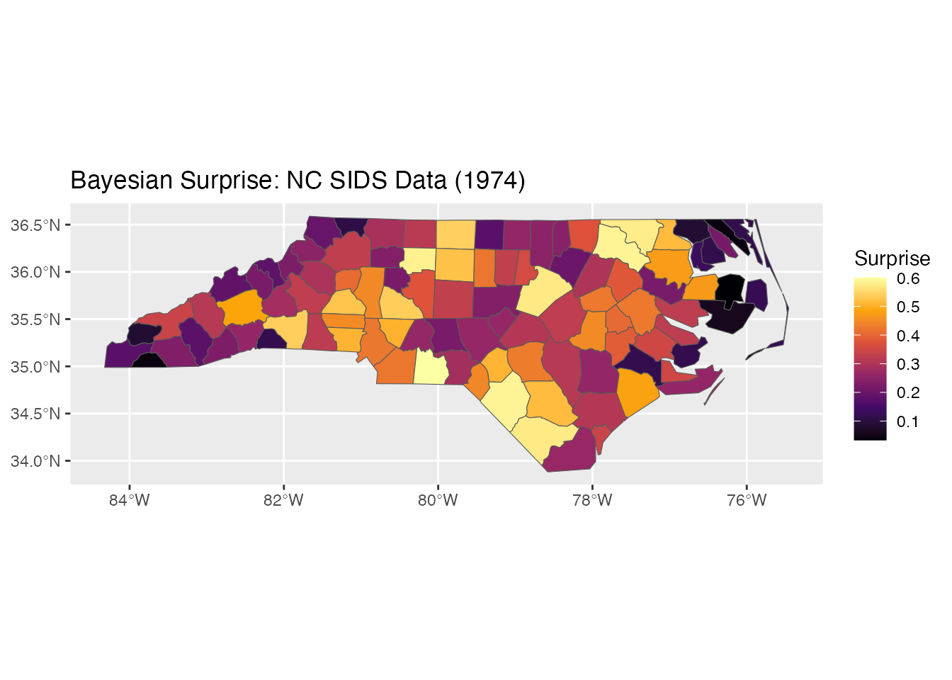

Map of North Carolina counties shaded by Bayesian surprise values.

# Plot signed surprise (shows direction of deviation)
ggplot(result) +
  geom_sf(aes(fill = signed_surprise)) +
  scale_fill_surprise_diverging() +
  labs(title = "Signed Surprise: Over/Under-representation")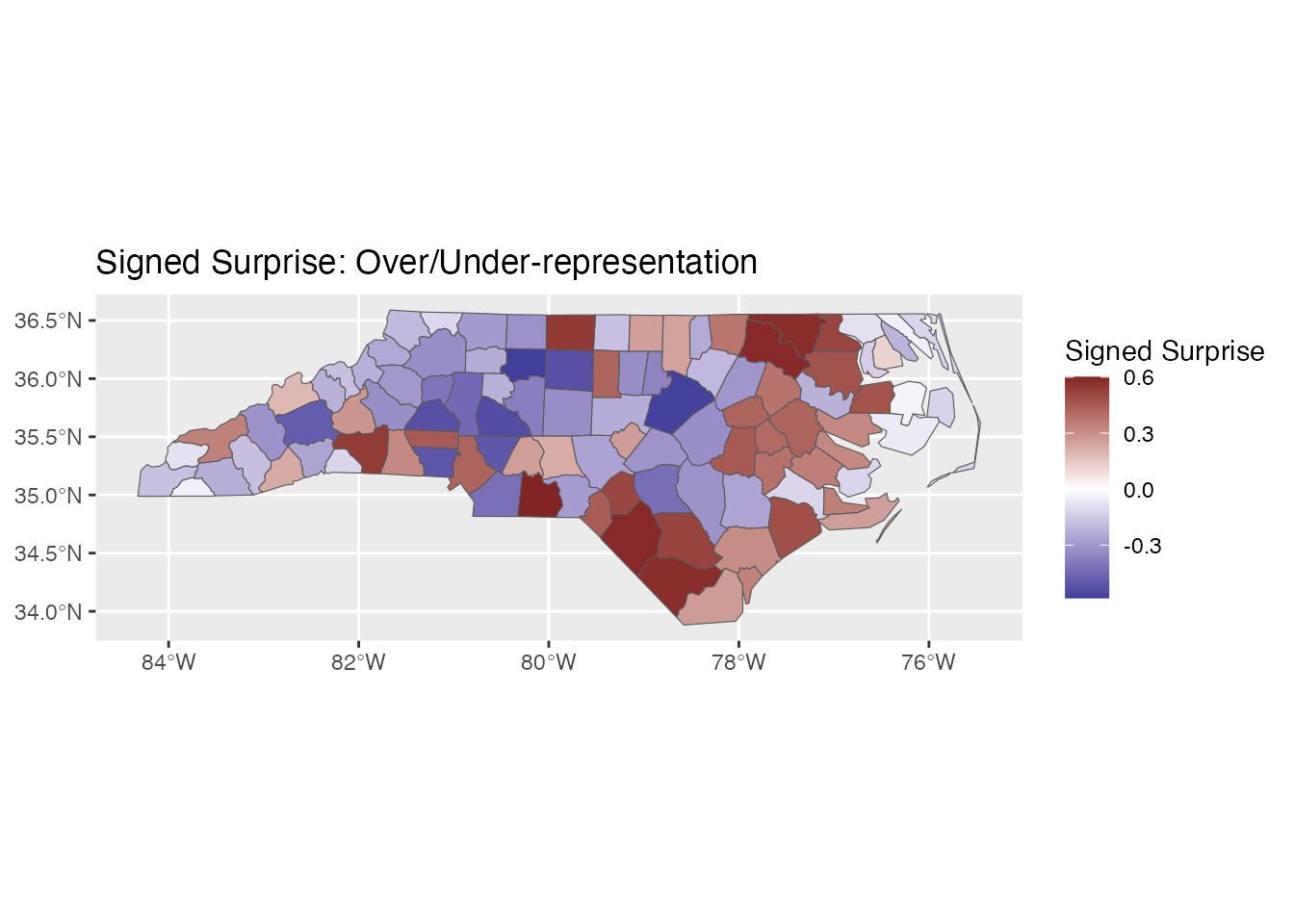

Map of North Carolina counties shaded by Bayesian surprise values.

Understanding the Output

The surprise() function returns an object containing:

surprise: Non-negative values indicating magnitude of surprise (in bits)
signed_surprise: Positive for over-representation, negative for under-representation
model_space: The models used and their posterior weights
posteriors: Per-observation posterior distributions

# Access surprise values directly
get_surprise(result, "surprise")[1:5]
#> [1] 0.1952858 0.1107616 0.2909684 0.1171487 0.5777373

# Access the model space
get_model_space(result)
#> <bs_model_space>
#>   Models: 3 
#>    1. Uniform (prior: 0.3333)
#>    2. Base Rate (prior: 0.3333)
#>    3. de Moivre Funnel (paper) (prior: 0.3333)

Customizing Models

By default, surprise() uses three models: - Uniform: All regions equally likely - Base Rate: Regions proportional to expected values - de Moivre Funnel: Accounts for sampling variance

You can customize the model space:

# Create custom model space
custom_space <- model_space(
  bs_model_uniform(),
  bs_model_baserate(nc$BIR74),
  bs_model_gaussian(),
  prior = c(0.2, 0.5, 0.3)  # Custom prior weights
)

result_custom <- surprise(nc, observed = SID74, expected = BIR74,
                          models = custom_space)
print(result_custom)
#> Bayesian Surprise Map
#> =====================
#> Models: 3 
#> Surprise range: 0.4351 to 2.3054 
#> Signed surprise range: -2.0136 to 2.3054 
#> 
#> Simple feature collection with 100 features and 16 fields
#> Geometry type: MULTIPOLYGON
#> Dimension:     XY
#> Bounding box:  xmin: -84.32385 ymin: 33.88199 xmax: -75.45698 ymax: 36.58965
#> Geodetic CRS:  NAD27
#> First 10 features:
#>     AREA PERIMETER CNTY_ CNTY_ID        NAME  FIPS FIPSNO CRESS_ID BIR74 SID74
#> 1  0.114     1.442  1825    1825        Ashe 37009  37009        5  1091     1
#> 2  0.061     1.231  1827    1827   Alleghany 37005  37005        3   487     0
#> 3  0.143     1.630  1828    1828       Surry 37171  37171       86  3188     5
#> 4  0.070     2.968  1831    1831   Currituck 37053  37053       27   508     1
#> 5  0.153     2.206  1832    1832 Northampton 37131  37131       66  1421     9
#> 6  0.097     1.670  1833    1833    Hertford 37091  37091       46  1452     7
#> 7  0.062     1.547  1834    1834      Camden 37029  37029       15   286     0
#> 8  0.091     1.284  1835    1835       Gates 37073  37073       37   420     0
#> 9  0.118     1.421  1836    1836      Warren 37185  37185       93   968     4
#> 10 0.124     1.428  1837    1837      Stokes 37169  37169       85  1612     1
#>    NWBIR74 BIR79 SID79 NWBIR79                       geometry  surprise
#> 1       10  1364     0      19 MULTIPOLYGON (((-81.47276 3... 0.6758063
#> 2       10   542     3      12 MULTIPOLYGON (((-81.23989 3... 0.5344499
#> 3      208  3616     6     260 MULTIPOLYGON (((-80.45634 3... 0.8628723
#> 4      123   830     2     145 MULTIPOLYGON (((-76.00897 3... 0.5277768
#> 5     1066  1606     3    1197 MULTIPOLYGON (((-77.21767 3... 1.8731869
#> 6      954  1838     5    1237 MULTIPOLYGON (((-76.74506 3... 1.6093786
#> 7      115   350     2     139 MULTIPOLYGON (((-76.00897 3... 0.4450687
#> 8      254   594     2     371 MULTIPOLYGON (((-76.56251 3... 0.4979554
#> 9      748  1190     2     844 MULTIPOLYGON (((-78.30876 3... 1.1184478
#> 10     160  2038     5     176 MULTIPOLYGON (((-80.02567 3... 0.9808319
#>    signed_surprise
#> 1       -0.6758063
#> 2       -0.5344499
#> 3       -0.8628723
#> 4       -0.5277768
#> 5        1.8731869
#> 6        1.6093786
#> 7       -0.4450687
#> 8       -0.4979554
#> 9        1.1184478
#> 10      -0.9808319

Next Steps

See vignette("model-types") for details on all five model types
See vignette("sf-workflow") for advanced spatial workflows
See vignette("ggplot2-visualization") for visualization options
See vignette("temporal-analysis") for time series and streaming data